
Prism: Seasonal-Trend Regression
Prism is a Python 3 package for spline-based regression and decomposition of time series with seasonal and trend components.
Installation
Prism requires Python 3.6 or greater. It was developed and tested on x86_64 systems running MacOS and Linux.
Dependencies
The package extra dependencies are listed in the files requirements.txt and requirements-conda.txt.
It is recommended to install those extra dependencies using Miniconda or
Anaconda. This
is not just a pure stylistic choice but comes with some hidden advantages, such as the linking to
Intel MKL library (a highly optimized BLAS library created by Intel).
>> conda install --channel=conda-forge --file=requirements-conda.txt
Quick Install
Prism can be installed very simply via the command:
>> pip install git+git://github.com/matthieumeo/prism.git@master#egg=prism
If you have previously activated your conda environment pip will install Prism in said environment. Otherwise it will install it in your base environment together with the various dependencies obtained from the file requirements.txt.
Developper Install
It is also possible to install Prism from the source for developpers:
>> git clone https://github.com/matthieumeo/prism
>> cd <repository_dir>/
>> pip install -e .
The package documentation can be generated with:
>> conda install sphinx=='2.1.*'
>> python3 setup.py build_sphinx -b singlehtml
Methods
Parametric Model
Consider an unknown signal \(f:\mathbb{R}\to \mathbb{R}\) of which we possess noisy samples
for some non-uniform sample times \(\{t_1,\ldots, t_L\}\subset \mathbb{R}\) and additive i.i.d. noise perturbations \(\epsilon_\ell\).
The SeasonalTrendRegression class assumes the following parametric form for \(f\):
where:
\(\sum_{n=1}^N \alpha_n=0\) (so as to enforce a zero-mean seasonal component, see note below),
\(\rho_{P}:[0, \Theta[\to \mathbb{R}\) is the \(\Theta\)-periodic Green function associated to the \(P\)-iterated derivative operator \(D^P\) [Periodic],
\(\psi_{Q}:\mathbb{R}\to \mathbb{R}\) is the causal Green function associated to the \(Q\)-iterated derivative operator \(D^Q\) [Green],
\(\theta_n:=(n-1)\Theta/N,\) and \(\eta_m:=R_{min}\,+\,m(R_{max}-R_{min})/(M+1),\) for some \(R_{min}<R_{max}\).
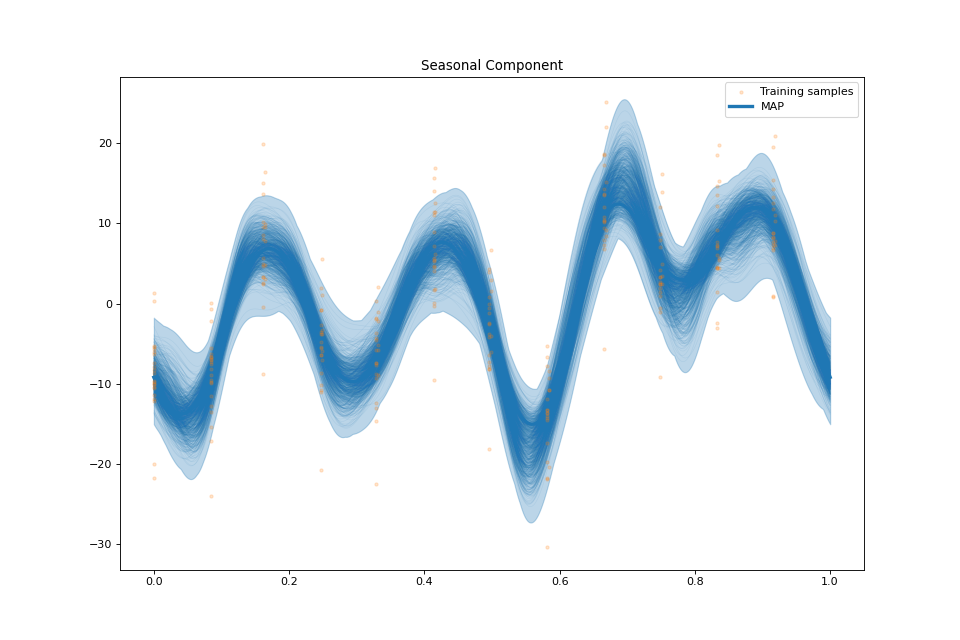
The seasonal component \(f_S(t):=\sum_{n=1}^N \alpha_n \rho_{P}(t-\theta_n)\) is a (zero mean) \(\Theta\)-periodic spline w.r.t. the iterated derivative operator \(D^k\) [Periodic]. It models short-term cyclical temporal variations of the signal \(f\).
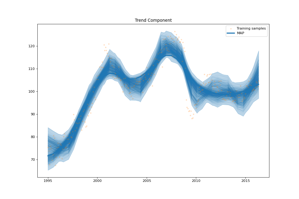
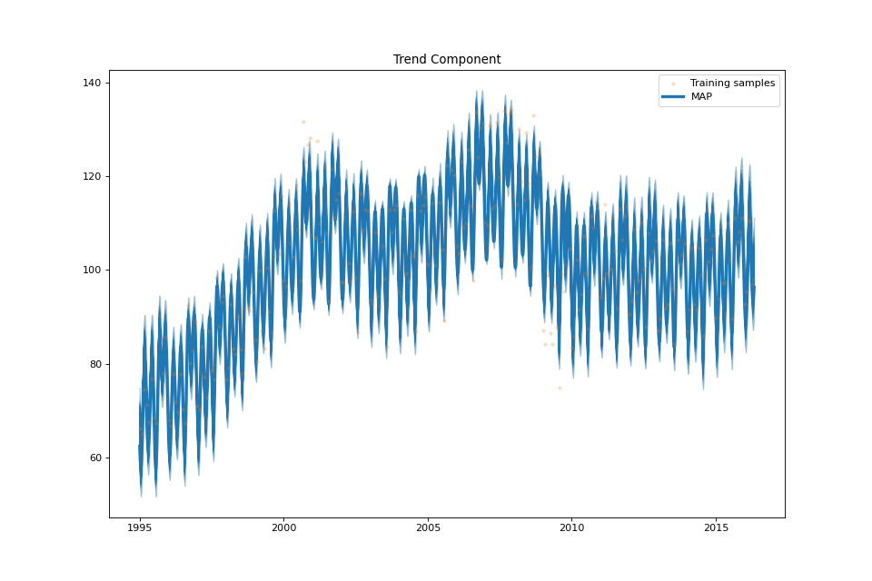
The trend component \(f_T(t):=\sum_{m=1}^M \beta_m \psi_{Q}(t-\eta_m)+\sum_{q=1}^{Q}\gamma_q t^{q-1}\) is a spline w.r.t. the iterated derivative operator \(D^Q\). It is the sum of a piecewise polynomial term \(\sum_{m=1}^M \beta_m \psi_{Q}(t-\eta_m)\) and a degree \(Q-1\) polynomial \(\sum_{q=1}^{Q}\gamma_q t^{q-1}\) [Splines]. It models long-term non-cyclical temporal variations of \(f\).
Note
Note that the mean of \(f\) could be assigned to the seasonal or trend component interchangeably, or even split between the two components. Constraining the seasonal component to have zero mean allows us to fix this unidentifiability issue.
Fitting Procedure
The method fit() recovers the coefficients \(\mathbf{a}=[\alpha_1,\ldots,\alpha_N]\in\mathbb{R}^N\), \(\mathbf{b}=[\beta_1,\ldots,\beta_M]\in\mathbb{R}^M\) and
\(\mathbf{c}=[\gamma_1,\ldots,\gamma_{Q}]\in\mathbb{R}^{Q}\) from the data \(\mathbf{y}=[y_1,\ldots,y_L]\in\mathbb{R}^L\)
as minima at posteriori (MAP) of the negative log-posterior distribution:
where:
\(p\in \{1,2\}\) is chosen according the the noise distribution (\(p=1\) in the presence of outliers),
\(\mathbf{K}\in\mathbb{R}^{L\times N}\) is given by: \(\mathbf{K}_{\ell n}=\rho_{P}(t_\ell-\theta_j)\),
\(\mathbf{L}\in\mathbb{R}^{L\times M}\) is given by: \(\mathbf{L}_{\ell m}=\psi_{Q}(t_\ell-\eta_m)\),
\(\mathbf{V}\in\mathbb{R}^{L\times Q}\) is a Vandermonde matrix given by: \(\mathbf{V}_{\ell q}=t^{q-1}_\ell\),
\(\lambda>0\) and \(\theta\in [0,1]\) are regularisation parameters,
\(\iota:\mathbb{R}\to\{0, +\infty\}\) is the indicator function returning \(0\) if the input is zero and \(+\infty\) otherwise.
If requested by the user, the penalty parameter \(\lambda\) can be learnt from the data by introducing a Gamma hyper-prior and finding the MAP of the posterior on \({\mathbf{a}}, {\mathbf{b}},{\mathbf{c}}\) and \(\lambda\) jointly [Tuning].
The \(R^2\)-score of the regression is provided by the method r2score().
Uncertainty Quantification
The method sample_credible_region() returns approximate marginal pointwise credible
intervals for the model parameters, the seasonal and trend components and their sum. This is achieved by sampling uniformly (via the hit-and-run algorithm) the
approximate highest density posterior credible region [Credible]:
\[C_{\xi}=\left\{({\mathbf{a}}, {\mathbf{b}},{\mathbf{c}})\in\mathbb{R}^N\times\mathbb{R}^M\times \mathbb{R}^Q: J({\mathbf{a}}, {\mathbf{b}},{\mathbf{c}})\leq J(\hat{\mathbf{a}}, \hat{\mathbf{b}}, \hat{\mathbf{c}}) + (N+M+Q) (\nu_\xi+1)\right\} \tag{3}\]
where \(\xi\in [0,1]\) is the confidence level associated to the credible region, \(\nu_\xi:=\sqrt{16\log(3/\xi)/(N+M+Q)}\), and \(J:\mathbb{R}^N\times\mathbb{R}^M\times \mathbb{R}^Q\to \mathbb{R}_+\) is the negative log-posterior in (3).
Approximate marginal pointwise credible intervals are then obtained by evaluating (1) (and the seasonal/trend components) for the various samples of \(C_{\xi}\) gathered and then taking the pointwise minima and maxima of all the sample curves.
Note that (3) can also be used for hypothesis testing on the parameters of the model (see method is_credible()
for more on the topic).
Reference Documentation
The seasonal-trend regression is performed by means of the SeasonalTrendRegression class described below:
-
class
SeasonalTrendRegression(sample_times: numpy.ndarray, sample_values: numpy.ndarray, period: numbers.Number, forecast_times: numpy.ndarray, seasonal_forecast_times: numpy.ndarray, nb_of_knots: Tuple[int, int] = (32, 32), spline_orders: Tuple[int, int] = (3, 2), penalty_strength: Optional[float] = None, penalty_tuning: bool = True, test_times: Optional[numpy.ndarray] = None, test_values: Optional[numpy.ndarray] = None, robust: bool = False, theta: float = 0.5, dtype: type = <class 'numpy.float64'>, tol: float = 0.001)¶ Bases:
objectSeasonal-trend regression of a noisy and non-uniform time series.
- Parameters
sample_times (numpy.ndarray) – Sample times \(\{t_1, \ldots, t_L\}\subset \mathbb{R}\).
sample_values (numpy.ndarray) – Observed values of the signal \(\{y_1, \ldots, y_L\}\subset \mathbb{R}\) at the sample times. Can be noisy.
period (Number) – Period \(\Theta>0\) for the seasonal component.
forecast_times (numpy.ndarray) – Unobserved times for forecasting of the signal and its trend component.
seasonal_forecast_times (numpy.ndarray) – Unobserved times in \([0,\Theta)\) for forecasting of the seasonal component.
nb_of_knots (Tuple[int, int]) – Number of knots \((N, M)\) for the seasonal and trend component respectively. High values of \(N\) and \(M\) can lead to numerical instability.
spline_orders (Tuple[int, int]) – Exponents \((P,Q)\) of the iterated derivative operators defining the splines involved in the seasonal and trend component respectively. Both parameters must be strictly bigger than one.
penalty_strength (Optional[Number]) – Value of the penalty strength \(\lambda\in \mathbb{R}_+\).
penalty_tuning (bool) – Whether or not the penalty strength \(\lambda\) should be learnt from the data.
test_times (Optional[numpy.ndarray]) – Optional test times to assess the regression performances.
test_values (Optional[numpy.ndarray]) – Optional test values to assess the regression performances.
robust (bool) – If
True, \(p=1\) is chosen for the data-fidelity term in (2), otherwise \(p=2\). Should be set toTruein the presence of outliers.theta (float) – Value of the balancing parameter \(\theta\in [0,1]\). Setting
thetaas 0 or 1 respectively removes the penalty on the seasonal or trend component in (2).dtype (type) – Types of the various numpy arrays involved in the estimation procedure.
tol (float) – Tolerance for computing Lipschitz constants. For experimented users only!
- Raises
ValueError – If
self.sample_times.size != self.sample_values.size,len(self.spline_orders) != 2,1 in self.spline_orders,len(self.nb_of_knots) != 2ornot 0 <= theta <= 1.
-
fit(max_outer_iterations: int = 10, max_inner_iterations: int = 10000, accuracy_parameter: float = 1e-05, accuracy_hyperparameter: float = 0.001, verbose: Optional[int] = None) → Tuple[numpy.ndarray, float]¶ Fit the model (1) by solving (2).
- Parameters
max_outer_iterations (int) – Maximum number of outer iterations for auto-tuning of the penalty strength \(\lambda\).
max_inner_iterations (int) – Maximum number of inner iterations when solving (2) with a fixed value of \(\lambda\).
accuracy_parameter (float) – Minimum relative improvement in the iterate of the numerical solver for (2).
accuracy_hyperparameter (float) – Minimum relative improvement of the penalty strength.
verbose (Optional[int]) – Verbosity level of the method.
- Returns
Estimates of \((\hat{\mathbf{a}}, \hat{\mathbf{b}}, \hat{\mathbf{c}})\) concatenated as a single array with size \(N+M+Q\) and the auto-tuned penalty parameter \(\lambda\).
- Return type
Tuple[np.ndarray, float]
-
r2score(dataset: str = 'training') → dict¶ \(R^2-score\) of the regression.
- Parameters
dataset (['training', 'test']) – Dataset on which to evaluate the \(R^2-score\).
- Returns
Dictionary containing the \(R^2-scores\) of the seasonal and trend components as well as the sum of the two.
- Return type
-
predict() → Tuple[numpy.ndarray, numpy.ndarray, numpy.ndarray]¶ Predict the values of the signal and its seasonal/trend components at times specified by the attributes
self.forecast_timesandself.seasonal_forecast_times.- Returns
Predicted values for the seasonal, trend and sum of the two respectively.
- Return type
Tuple[np.ndarray, np.ndarray, np.ndarray]
-
sample_credible_region(n_samples: float = 100000.0, credible_lvl: float = 0.01, return_samples: bool = False, seed: int = 1, subsample_by: int = 100) → Tuple[dict, dict, Optional[dict]]¶ Sample approximate credible region and returns pointwise marginal credible intervals.
- Parameters
n_samples (float) – Number of samples.
credible_lvl (float) – Credible level \(\xi\in [0,1]\).
return_samples (bool) – If
True, return the samples on top of the pointwise marginal credible intervals.seed (int) – Seed for the pseudo-random number generator.
subsample_by – Subsampling factor (1 every
subsample_bysamples are stored ifreturn_samples==True).
- Returns
Dictionaries with keys {‘coeffs’, ‘seasonal’, ‘trend’, ‘sum’}. The values associated to the keys of the first two dictionaries are the minimum and maximum of the credible intervals of the corresponding component. The values associated to the keys of the last dictionary are arrays containing credible samples of the corresponding component.
- Return type
-
is_credible(coeffs: numpy.ndarray, credible_lvl: Optional[float] = None, gamma: Optional[float] = None) → Tuple[bool, bool, float]¶ Test whether a set of coefficients are credible for a given confidence level.
- Parameters
- Returns
The set of coefficients are credible if the product of the first two output is 1. The last output is for internal use only.
- Return type
-
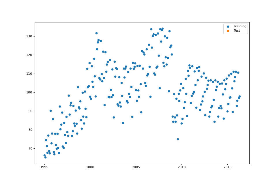
plot_data(fig: Optional[int] = None, test_set: bool = True)¶ Plot the training and test datasets.
- Parameters
fig (Optional[int]) – Figure handle. If
Nonecreates a new figure.test_set – Optional test dataset.
-
plot_green_functions(fig: Optional[int] = None, component: str = 'trend')¶ Plot the shifted Green functions involved in the parametric model (1).
- Parameters
fig (Optional[int]) – Figure handle. If
Nonecreates a new figure.component (['seasonal', 'trend']) – Component for which the shifted Green functions should be plotted.
-
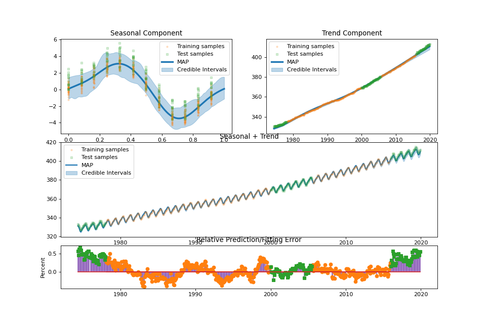
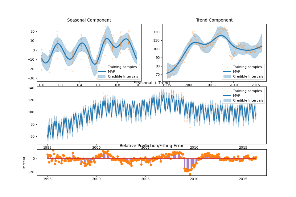
summary_plot(fig: Optional[int] = None, min_values: Optional[dict] = None, max_values: Optional[dict] = None)¶ Plot the result of the regression.
- Parameters
fig (Optional[int]) – Figure handle. If
Nonecreates a new figure.min_values (Optional[dict]) – Minimum of the pointwise marginal credible intervals for the various components. Output of
sample_credible_region().max_values (Optional[dict]) – Maximum of the pointwise marginal credible intervals for the various components. Output of
sample_credible_region().
-
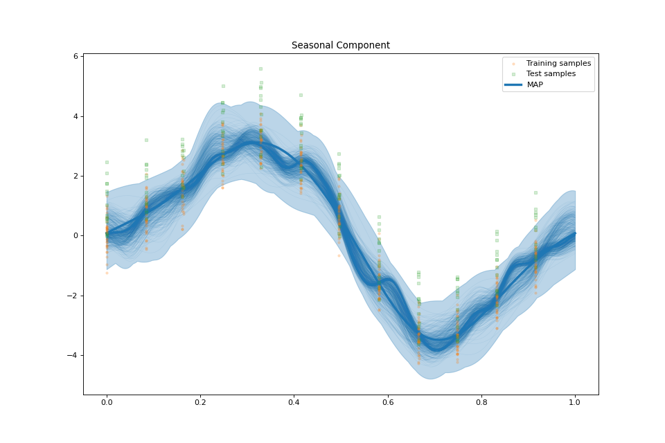
plot_seasonal_component(fig: Optional[int] = None, samples_seasonal: Optional[numpy.ndarray] = None, min_values: Optional[numpy.ndarray] = None, max_values: Optional[numpy.ndarray] = None)¶ Plot the seasonal component.
- Parameters
fig (Optional[int]) – Figure handle. If
Nonecreates a new figure.samples_seasonal (Optional[np.ndarray] = None) – Sample curves for the seasonal component. Output of
sample_credible_region().min_values (Optional[np.ndarray]) – Minimum of the pointwise marginal credible intervals for the seasonal component. Output of
sample_credible_region().max_values (Optional[np.ndarray]) – Maximum of the pointwise marginal credible intervals for the seasonal component. Output of
sample_credible_region().
-
plot_trend_component(fig: Optional[int] = None, samples_trend: Optional[numpy.ndarray] = None, min_values: Optional[numpy.ndarray] = None, max_values: Optional[numpy.ndarray] = None)¶ Plot the trend component.
- Parameters
fig (Optional[int]) – Figure handle. If
Nonecreates a new figure.samples_trend (Optional[np.ndarray] = None) – Sample curves for the trend component. Output of
sample_credible_region().min_values (Optional[np.ndarray]) – Minimum of the pointwise marginal credible intervals for the trend component. Output of
sample_credible_region().max_values (Optional[np.ndarray]) – Maximum of the pointwise marginal credible intervals for the trend component. Output of
sample_credible_region().
-
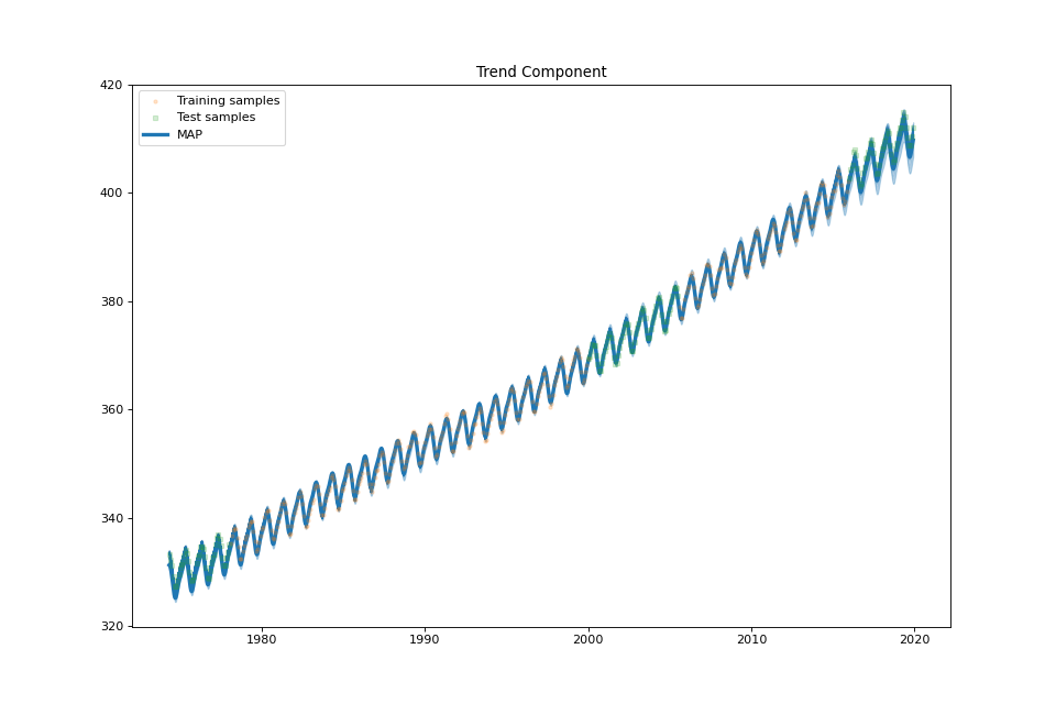
plot_sum(fig: Optional[int] = None, samples_sum: Optional[numpy.ndarray] = None, min_values: Optional[numpy.ndarray] = None, max_values: Optional[numpy.ndarray] = None)¶ Plot the sum of the seasonal and trend component.
- Parameters
fig (Optional[int]) – Figure handle. If
Nonecreates a new figure.samples_sum (Optional[np.ndarray] = None) – Sample curves for the sum of the two component. Output of
sample_credible_region().min_values (Optional[np.ndarray]) – Minimum of the pointwise marginal credible intervals for the sum of the two components. Output of
sample_credible_region().max_values (Optional[np.ndarray]) – Maximum of the pointwise marginal credible intervals for the sum of the two components. Output of
sample_credible_region().
Examples
Atmospheric CH4
import numpy as np
import matplotlib.pyplot as plt
from prism import SeasonalTrendRegression
from prism import ch4_mlo_dataset
plt.rcParams['figure.figsize'] = [12, 8]
plt.rcParams['figure.dpi'] = 100
data, data_test = ch4_mlo_dataset()
period = 1
sample_times = data.time_decimal.values
sample_values = data.value.values
test_times = data_test.time_decimal.values
test_values = data_test.value.values
forecast_times = np.linspace(test_times.min(), test_times.max(), 4096)
seasonal_forecast_times = np.linspace(0, period, 1024)
streg = SeasonalTrendRegression(sample_times=sample_times, sample_values=sample_values, period=period,
forecast_times=forecast_times, seasonal_forecast_times=seasonal_forecast_times,
nb_of_knots=(32, 32), spline_orders=(3, 2), penalty_strength=1, penalty_tuning=False,
test_times=test_times, test_values=test_values, robust=False, theta=0.5)
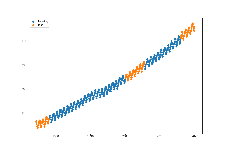
streg.plot_data()
xx, mu = streg.fit(verbose=1)
r2score = streg.r2score()
min_values, max_values, samples = streg.sample_credible_region(return_samples=True, subsample_by=1000)
streg.summary_plot(min_values=min_values, max_values=max_values)
streg.plot_seasonal_component(min_values=min_values['seasonal'], max_values=max_values['seasonal'],
samples_seasonal=samples['seasonal'])
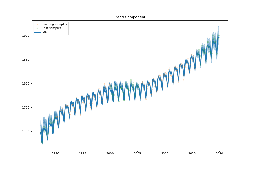
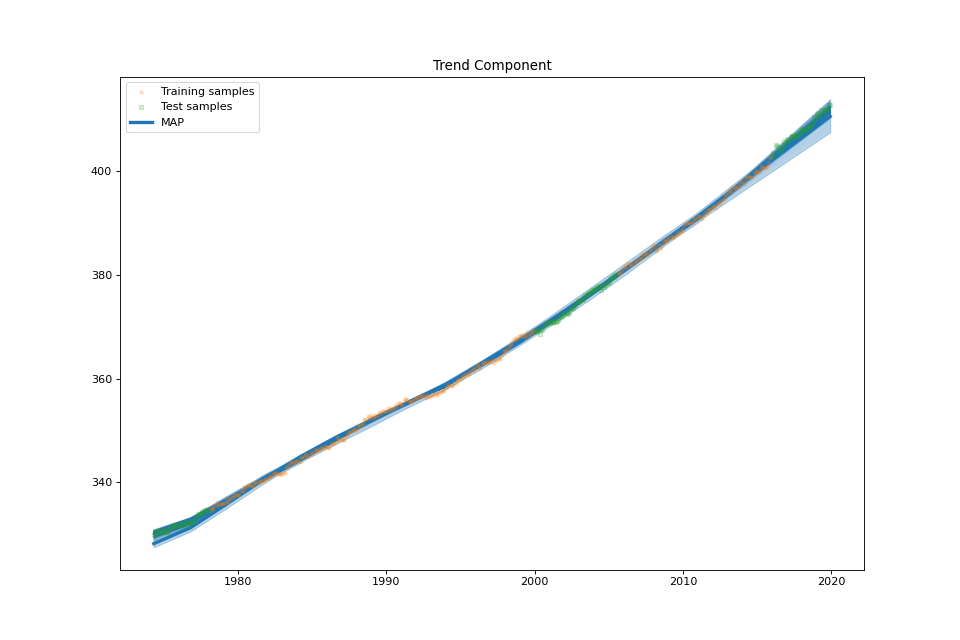
streg.plot_trend_component(min_values=min_values['trend'], max_values=max_values['trend'],
samples_trend=samples['trend'])
streg.plot_sum(min_values=min_values['sum'], max_values=max_values['sum'], samples_sum=samples['sum'])
Atmospheric CO2
import numpy as np
import matplotlib.pyplot as plt
from prism import SeasonalTrendRegression
from prism import co2_mlo_dataset

plt.rcParams['figure.figsize'] = [12, 8]
plt.rcParams['figure.dpi'] = 100

data, data_test = co2_mlo_dataset()

period = 1
sample_times = data.time_decimal.values
sample_values = data.value.values
test_times = data_test.time_decimal.values
test_values = data_test.value.values
forecast_times = np.linspace(test_times.min(), test_times.max(), 4096)
seasonal_forecast_times = np.linspace(0, period, 1024)

streg = SeasonalTrendRegression(sample_times=sample_times, sample_values=sample_values, period=period,
                                forecast_times=forecast_times, seasonal_forecast_times=seasonal_forecast_times,
                                nb_of_knots=(32, 16), spline_orders=(3, 2), penalty_strength=1, penalty_tuning=True,
                                test_times=test_times, test_values=test_values, robust=False, theta=0.5)
streg.plot_data()
xx, mu = streg.fit(verbose=1)
min_values, max_values, samples = streg.sample_credible_region(return_samples=True)
streg.summary_plot(min_values=min_values, max_values=max_values)
streg.plot_seasonal_component(min_values=min_values['seasonal'], max_values=max_values['seasonal'],
                              samples_seasonal=samples['seasonal'])
streg.plot_trend_component(min_values=min_values['trend'], max_values=max_values['trend'],
                           samples_trend=samples['trend'])
streg.plot_sum(min_values=min_values['sum'], max_values=max_values['sum'], samples_sum=samples['sum'])
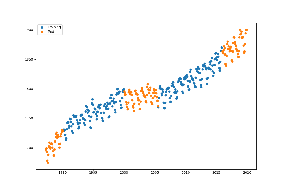
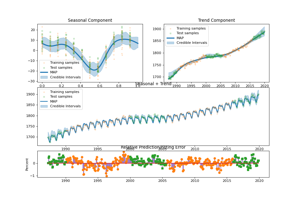
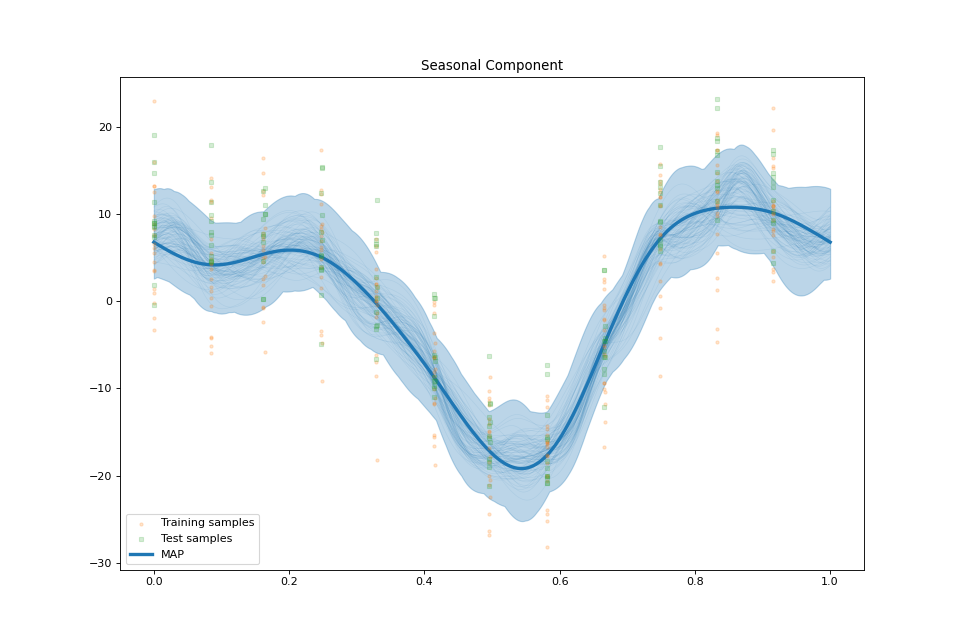
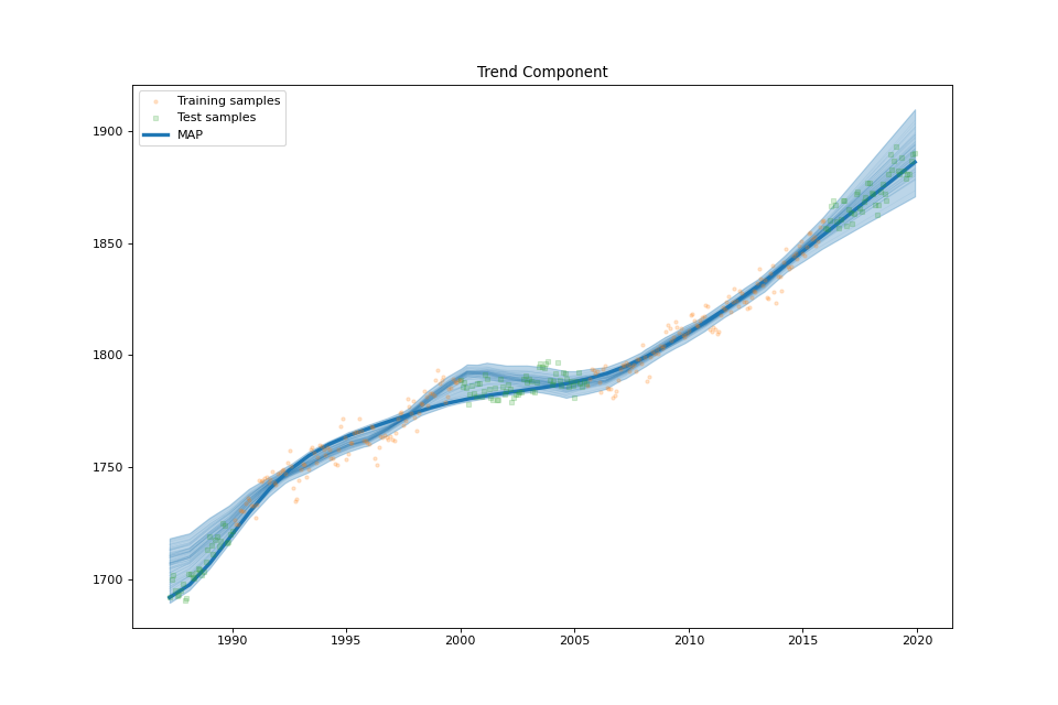
US Electronic Equipment
import numpy as np
import matplotlib.pyplot as plt
from prism import SeasonalTrendRegression
from prism import elec_equip_dataset

plt.rcParams['figure.figsize'] = [12, 8]
plt.rcParams['figure.dpi'] = 100

data = elec_equip_dataset()

period = 1
sample_times = data.time_decimal.values
sample_values = data.value.values
forecast_times = np.linspace(sample_times.min(), sample_times.max(), 4096)
seasonal_forecast_times = np.linspace(0, period, 1024)

streg = SeasonalTrendRegression(sample_times=sample_times, sample_values=sample_values, period=period,
                                forecast_times=forecast_times, seasonal_forecast_times=seasonal_forecast_times,
                                nb_of_knots=(32, 40), spline_orders=(3, 2), penalty_strength=1, penalty_tuning=True,
                                test_times=None, test_values=None, robust=False, theta=0.5)
streg.plot_data()
xx, mu = streg.fit(verbose=1)
min_values, max_values, samples = streg.sample_credible_region(return_samples=True)
streg.summary_plot(min_values=min_values, max_values=max_values)
streg.plot_seasonal_component(min_values=min_values['seasonal'], max_values=max_values['seasonal'],
                              samples_seasonal=samples['seasonal'])
streg.plot_trend_component(min_values=min_values['trend'], max_values=max_values['trend'],
                           samples_trend=samples['trend'])
streg.plot_sum(min_values=min_values['sum'], max_values=max_values['sum'], samples_sum=samples['sum'])
References
- Periodic
Fageot, Julien, and Matthieu Simeoni. “TV-based reconstruction of periodic functions.” Inverse Problems 36.11 (2020): 115015.
- Splines
Gupta, Harshit, Julien Fageot, and Michael Unser. “Continuous-domain solutions of linear inverse problems with Tikhonov versus generalized TV regularization.” IEEE Transactions on Signal Processing 66.17 (2018): 4670-4684.
- Green
Unser, Michael, Julien Fageot, and John Paul Ward. “Splines are universal solutions of linear inverse problems with generalized TV regularization.” SIAM Review 59.4 (2017): 769-793.
- Tuning
Pereyra, Marcelo, José M. Bioucas-Dias, and Mário AT Figueiredo. “Maximum-a-posteriori estimation with unknown regularisation parameters.” 2015 23rd European Signal Processing Conference (EUSIPCO). IEEE, 2015.
- Credible
Pereyra, Marcelo. “Maximum-a-posteriori estimation with Bayesian confidence regions.” SIAM Journal on Imaging Sciences 10.1 (2017): 285-302.
