Spherical Linear Operators
Module: pycsphere.linop
Common spherical linear operators.
Convolution/Pooling
|
Zonal spherical convolution. |
|
Spherical pooling operator. |
Differential Operators
|
Discrete spherical Laplacian. |
|
Discrete spherical gradient. |
Transforms
|
Spherical Harmonic Transform (SHT). |
|
Fourier Legendre Transform (FLT). |
-
class
ZonalSphericalConvolution(size: int, spectral_window: Optional[numpy.ndarray] = None, zonal_filter: Optional[numpy.ndarray] = None, n_filter: Optional[int] = None, sigma: Optional[float] = None, use_weights: bool = False)[source]¶ Bases:
pycsou.core.linop.LinearOperatorZonal spherical convolution.
Compute the convolution between a bandlimited zonal kernel \(\psi(\langle\mathbf{r},\mathbf{s}\rangle)\) and a bandlimited spherical map \(f(\mathbf{r})\):
\[\left\{\psi\ast f\right\}(\mathbf{r})=\int_{\mathbb{S}^{2}}\psi(\langle\mathbf{r},\mathbf{s}\rangle)f(\mathbf{s})\,d\mathbf{s},\quad \forall \mathbf{r}\in\mathbb{S}^{2}.\]Examples
import healpy as hp
import numpy as np
from pycsphere.linop import SHT, FLT, ZonalSphericalConvolution
import matplotlib.pyplot as plt
from scipy.interpolate import interp1d

n_max = 30
nside = SHT.nmax2nside(n_max)
rng = np.random.default_rng(0)
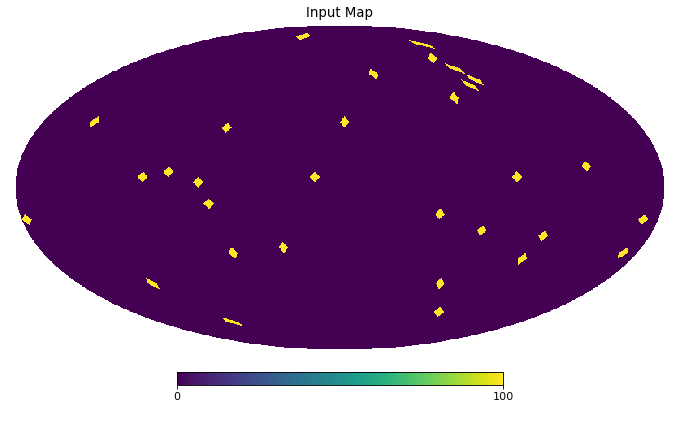
map_in = 100 * rng.binomial(n=1, p=0.01, size=int(hp.nside2npix(nside=nside)))
n=np.arange(2000)
spectral_window=1/(100+n*(n+1))**2
flt=FLT(n_max=1999, t=np.linspace(-1,1,2048))
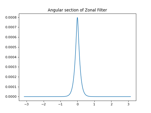
zonal_filter=flt.adjoint(spectral_window)
zonal_filter_interp=interp1d(flt.t, zonal_filter, assume_sorted=True)
convOp = ZonalSphericalConvolution(size=map_in.size, spectral_window=spectral_window)
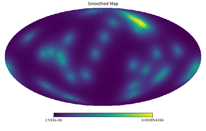
map_smoothed = convOp(map_in)
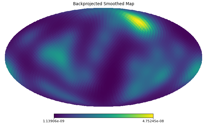
map_bismoothed = convOp.adjoint(map_smoothed)
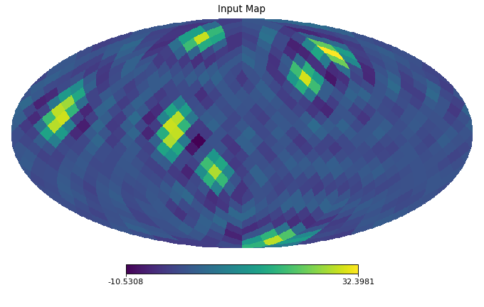
hp.mollview(map=map_in, title='Input Map', cmap='viridis')
plt.figure()
theta=np.linspace(-np.pi, np.pi, 1024)
plt.plot(theta, zonal_filter_interp(np.cos(theta)))
plt.title('Angular section of Zonal Filter')
hp.mollview(map=map_smoothed, title='Smoothed Map', cmap='viridis')
hp.mollview(map=map_bismoothed, title='Backprojected Smoothed Map', cmap='viridis')
Notes
The
ZonalSphericalConvolutionoperator is self-adjoint and can be computed efficiently in the spherical harmonic domain:\[\begin{split}\left\{\psi\ast f\right\}(\mathbf{r})&=\int_{\mathbb{S}^{2}}\psi(\langle\mathbf{r},\mathbf{s}\rangle)f(\mathbf{s})\,d\mathbf{s}\\ &= \sum_{n=0}^N\hat{\psi}_n\sum_{m=-n}^n \hat{f}_n^m Y_n^m(\mathbf{r}),\quad \forall \mathbf{r}\in\mathbb{S}^{2},\end{split}\]where \(N\) is the maximum between the bandwidth of \(f\) and \(\psi\). To perform this computation, we use the routine
healpy.sphtfunc.smoothing()which assumes a RING-ordered HEALPix discretisation of \(f\).Warning
This class is for real spherical maps \(f\) only.
Using this operator on non-bandlimited spherical maps \(f\) incurs aliasing.
HEALPix maps used as inputs must be RING ordered.
See also
SphericalHarmonicTransform,FourierLegendreTransform,BiZonalSphericalConvolution-
__init__(size: int, spectral_window: Optional[numpy.ndarray] = None, zonal_filter: Optional[numpy.ndarray] = None, n_filter: Optional[int] = None, sigma: Optional[float] = None, use_weights: bool = False)[source]¶ - Parameters
size (int) – Size of the RING-ordered, HEALPix-discretised sherical map \(f\).
spectral_window (Optional[np.ndarray]) – Fourier-Legendre coefficients \(\hat{\psi}_n\) of the zonal filter. Overrides
zonal_filter,n_filterandsigma.zonal_filter (Optional[np.ndarray]) – Zonal filter \(\psi\) discretised on [-1,1]. Overrides
sigma.n_filter (Optional[int]) – Bandwidth of the zonal filter \(\psi\). Only used if
zonal_filteris specified.sigma (float) – Standard deviation of a Gaussian filter in radians.
use_weights (bool) – If
True, use the ring weighting quadrature rule when computing the spherical harmonic transform.
Notes
The zonal filter can be specified in three ways:
Via its Fourier-Legendre coefficients (keyword
spectral_window).Via its discretisation on [-1,1] and its bandwidth (keywords
zonal_filterandn_filter).As a spherical Gaussian filter with standard deviation
sigmain radians.
If keywords from multiple scenarios are used, 1. overrides 2. and 3. and 2. overrides 3.
-
class
SphericalPooling(nside_in: int, nside_out: int, order_in: str = 'RING', order_out: str = 'RING', pooling_func: str = 'mean', dtype: type = <class 'numpy.float64'>)[source]¶ Bases:
pycsou.core.linop.LinearOperatorSpherical pooling operator.
Pool an HEALPix map by summing/averaging children pixels nested in a common superpixel.
Examples
import healpy as hp
import numpy as np
from pycsphere.linop import SphericalPooling

nside = 16
rng = np.random.default_rng(0)
map_in = rng.binomial(n=1, p=0.2, size=hp.nside2npix(nside=nside))
map_in = hp.smoothing(map_in, sigma=10 * np.pi / 180)
pool = SphericalPooling(nside_in=nside, nside_out=8, pooling_func='sum')
pooled_map = pool(map_in)
backprojected_map = pool.adjoint(pooled_map)
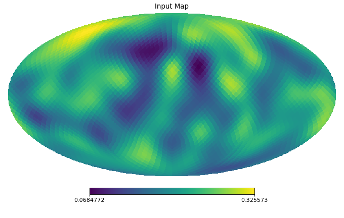
hp.mollview(map=map_in, title='Input Map', cmap='viridis')
hp.mollview(map=pooled_map, title='Pooled Map', cmap='viridis')
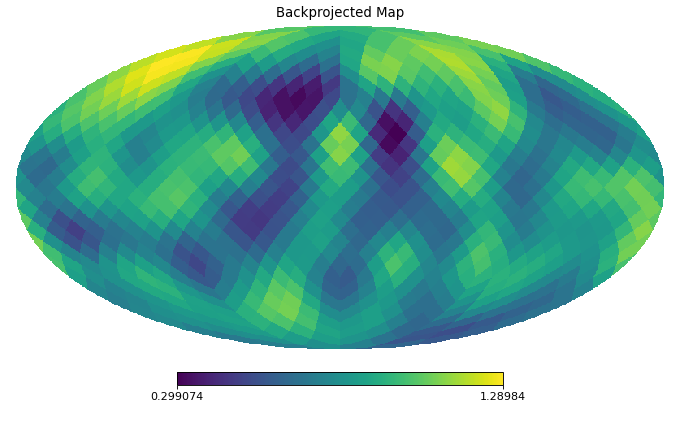
hp.mollview(map=backprojected_map, title='Backprojected Map', cmap='viridis')
Notes
Pooling is performed via the function
healpy.pixelfunc.ud_grade()from Healpy. The adjoint (unpooling) is performed by assigning the value of the superpixels through the pooling function (e.g. mean, sum) to each children pixels of the superpixels.-
__init__(nside_in: int, nside_out: int, order_in: str = 'RING', order_out: str = 'RING', pooling_func: str = 'mean', dtype: type = <class 'numpy.float64'>)[source]¶ - Parameters
nside_in (int) – Parameter NSIDE of the input HEALPix map.
nside_out (int) – Parameter NSIDE of the pooled HEALPix map.
order_in (str ['RING', 'NESTED']) – Ordering of the input HEALPix map.
order_out (str ['RING', 'NESTED']) – Ordering of the pooled HEALPix map.
pooling_func (str ['mean', 'sum']) – Pooling function.
dtype (type) – Data type of the linear operator.
- Raises
ValueError – If
nside_out >= nside_in.
-
-
class
DiscreteSphericalLaplacian(point_set: pycsphere.mesh.SphericalPointSet, dtype: type = <class 'numpy.float64'>)[source]¶ Bases:
pycgsp.linop.diff.GraphLaplacianDiscrete spherical Laplacian.
Finite-difference approximation of the continuous spherical Laplacian for a map defined over a
SphericalPointSet.Examples
import healpy as hp
import numpy as np
from pycsphere.mesh import HEALPixPointSet
from pycsphere.linop import DiscreteSphericalLaplacian

nside = 16
rng = np.random.default_rng(0)
map_in = rng.binomial(n=1, p=0.005, size=hp.nside2npix(nside=nside))
map_in = hp.smoothing(map_in, sigma=10 * np.pi / 180)
laplacian = DiscreteSphericalLaplacian(point_set=HEALPixPointSet(nside=nside))
map_d2 = laplacian(map_in)
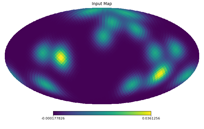
hp.mollview(map=map_in, title='Input Map', cmap='viridis')
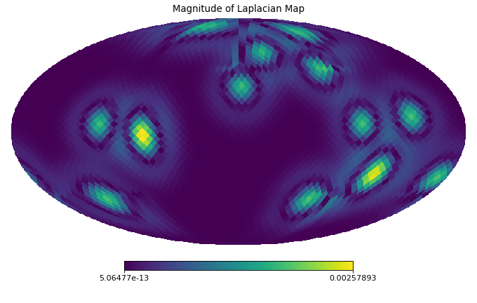
hp.mollview(map=np.abs(map_d2), title='Magnitude of Laplacian Map', cmap='viridis')
Notes
The discrete Laplacian is computed as the Laplacian of the spherical point set’s graph Pycsou-gsp tessellation graphs using
pycgsp.linop.diff.GraphLaplacian.-
__init__(point_set: pycsphere.mesh.SphericalPointSet, dtype: type = <class 'numpy.float64'>)[source]¶ - Parameters
point_set (SphericalPointSet) – Spherical point set on which the signal is defined.
dtype (type) – Input type.
-
-
class
DiscreteSphericalGradient(point_set: pycsphere.mesh.SphericalPointSet, dtype: type = <class 'numpy.float64'>)[source]¶ Bases:
pycgsp.linop.diff.GraphGradientDiscrete spherical gradient.
Finite-difference approximation of the continuous spherical gradient for a map defined over a
SphericalPointSet.Notes
The discrete gradient is computed as the gradient of the spherical point set’s graph (see Pycsou-gsp tessellation graphs) using
pycgsp.linop.diff.GraphGradient.-
__init__(point_set: pycsphere.mesh.SphericalPointSet, dtype: type = <class 'numpy.float64'>)[source]¶ - Parameters
point_set (SphericalPointSet) – Spherical point set on which the signal is defined.
dtype (type) – Input type.
-
-
class
SphericalHarmonicTransform(n_max: int, use_weights: bool = False, verbose: bool = False)[source]¶ Bases:
pycsou.core.linop.LinearOperatorSpherical Harmonic Transform (SHT).
Compute the spherical harmonic transform of a real bandlimited spherical function \(f:\mathbb{S}^2\to\mathbb{R}\).
Examples
import healpy as hp
import numpy as np
from pycsphere.linop import SHT
import matplotlib.pyplot as plt

n_max = 20
nside = SHT.nmax2nside(n_max)
rng = np.random.default_rng(0)
map_in = 100 * rng.binomial(n=1, p=0.01, size=int(hp.nside2npix(nside=nside)))
map_in = hp.smoothing(map_in, beam_window=np.ones(shape=(3*n_max//4,)))
sht = SHT(n_max=n_max)
anm = sht(map_in)
synth_map = sht.adjoint(anm)
hp.mollview(map=map_in, title='Input Map', cmap='viridis')
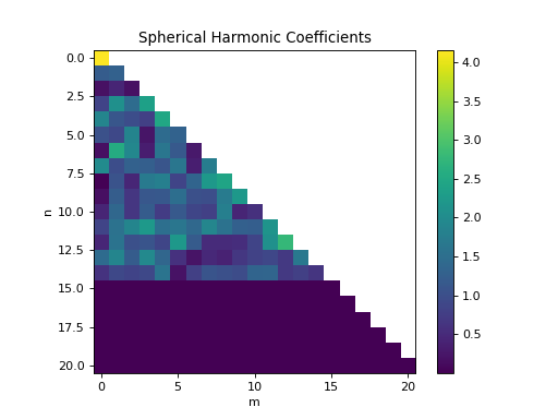
sht.plot_anm(anm)
hp.mollview(map=synth_map, title='Synthesised Map', cmap='viridis')
Notes
Every function \(f\in\mathcal{L}^2(\mathbb{S}^{2})\) admits a spherical Fourier expansion given by
\[f\stackrel{\mathcal{L}^2}{=}\sum_{n=0}^{+\infty}\sum_{m=-n}^{n} \,\hat{a}_n^m \,Y_n^m,\]where the spherical harmonic coefficients \(\{\hat{a}_n^m\}\subset\mathbb{C}\) of \(f\) are given by the Spherical Harmonic Transform:
\[\hat{a}_n^m=\int_{0}^\pi\int_{-\pi}^\pi f(\phi,\theta) \overline{Y_n^m(\phi,\theta)} \,\sin(\theta)d\phi d\theta.\]The functions \(Y_n^m:[-\pi,\pi[\times [0,\pi]\to \mathbb{C}\) are called the spherical harmonics and are given by:
\[Y_n^m(\phi,\theta):=\sqrt{\frac{(2n+1)(n-m)!}{4\pi (n+m)!}}P_n^m(\cos(\theta))e^{j m\phi}, \;\forall (\phi,\theta)\in[-\pi,\pi[\times [0,\pi],\]where \(P_n^m:[-1,1]\rightarrow \mathbb{R}\) denote the associated Legendre functions (see Chapter 1 of [Rafaely]).
For bandlimited functions of order \(N\in\mathbb{N}\) (\(|\hat{a}_n^m|=0\forall n>N\)), the spherical harmonic coefficients can be approximated very accurately via the spherical quadrature rule (see HEALPix help):
\[\hat{a}_n^m=\frac{4\pi}{N_{pix}}\sum_{p=1}^{N_{pix}} f(\phi_p,\theta_p) \overline{Y_n^m(\phi_p,\theta_p)}\]assuming a HEALPix spherical point set \(\left\{\mathbf{r}_p(\phi_p,\theta_p)\in\mathbb{S}^2, p=1, \ldots, N_{pix}=12N_{side}^2\right\}\) with \(2 N_{side}<N\leq 3 N_{side}-1\). The spherical harmonic transform and its inverse (adjoint) are computed with the routines
healpy.sphtfunc.map2alm()andhealpy.sphtfunc.alm2map()which compute the spherical harmonics efficiently via recurrence relations for Legendre polynomials on co-latitudes, and Fast Fourier Transforms on longitudes (see HEALPix help). If accuracy is a concern, ring-based quadrature rules can also be used with the keyworduse_weights=True.Warning
This class is for real spherical maps only. Complex spherical maps are not supported yet by the routines
healpy.sphtfunc.map2alm()andhealpy.sphtfunc.alm2map()which compute only half of the spherical harmonic coefficients, assuming symmetry.Using this operator on non-bandlimited spherical maps incurs aliasing.
HEALPix maps used as inputs must be RING ordered.
See also
-
classmethod
nmax2nside(n_max: int) → int[source]¶ Compute the critical HEALPix NSIDE parameter for a given bandwidth
n_max.
-
__init__(n_max: int, use_weights: bool = False, verbose: bool = False)[source]¶ - Parameters
n_max (int) – Bandwidth of the map.
use_weights (bool) –
If
True, use ring-based quadrature weights (more accurate), otherwise use uniform quadrature weights. See HEALPix help for more information.verbose (bool) – If
Trueprints diagnostic information.
-
adjoint(anm: numpy.ndarray, nside: Optional[int] = None) → numpy.ndarray[source]¶ Compute the inverse spherical harmonic transform.
- Parameters
anm (np.ndarray) – Spherical harmonic coefficients \(\{\hat{a}_n^m\}\subset\mathbb{C}\).
- Returns
Synthesised bandlimited spherical map discretised on a critical RING ordered HEALPix mesh.
- Return type
np.ndarray
-
anm2cn(anm: numpy.ndarray) → numpy.ndarray[source]¶ Compute the angular power spectrum.
The angular power spectrum is defined as:
\[\hat{c}_n:=\frac{1}{2n+1}\sum_{m=-n}^n |\hat{a}_n^m|^2, \quad n\in \mathbb{N}.\]- Parameters
anm (np.ndarray) – Spherical harmonic coefficients \(\{\hat{a}_n^m\}\subset\mathbb{C}\).
- Returns
- Return type
The angular power spectrum coefficients \(\hat{c}_n\).
-
anm_triangle(anm: numpy.ndarray) → numpy.ndarray[source]¶ Arrange the spherical harmonic coefficients in a lower-triangular matrix where each row represents a level \(n\).
- Parameters
anm (np.ndarray) – Spherical harmonic coefficients.
- Returns
Spherical harmonic coefficients arranged in a lower-triangular matrix.
- Return type
np.ndarray
-
plot_anm(anm: numpy.ndarray, cmap: str = 'viridis', cast: Callable = <ufunc 'absolute'>)[source]¶ Plot the spherical harmonic coefficients.
- Parameters
anm (np.ndarray) – Spherical harmonic coefficients.
cmap (str) – Colormap.
cast (Callable) – Function to cast the complex coefficients into real coefficients (e.g.
np.abs,np.real,np.imag…)
-
SHT
-
class
FourierLegendreTransform(n_max: int, t: numpy.ndarray, dtype: type = <class 'numpy.float64'>)[source]¶ Bases:
pycsou.core.linop.LinearOperatorFourier Legendre Transform (FLT).
Compute the Fourier Legendre Transform of a function \(f:[-1,1]\to\mathbb{C}\). This is useful for computing the spherical harmonics coefficients of spherical zonal functions of the form \(g(\mathbf{r})=f(\langle\mathbf{r}, \mathbf{s}\rangle)\). Indeed, for such functions, we have:
\[\hat{g}_n^m=\hat{f}_n \sqrt{\frac{2n+1}{4\pi}}\delta_n^0, \quad \forall n,m,\]where \(\hat{f}_n\) are the Fourier-Legendre coefficients of \(f\). Moreover, from the Fourier-Legendre expansion we have also:
\[f(\langle\mathbf{r}, \mathbf{s}\rangle)=\sum_{n=0}^{+\infty} \hat{f}_n\frac{2n+1}{4\pi} P_n(\langle\mathbf{r}, \mathbf{s}\rangle).\]Examples
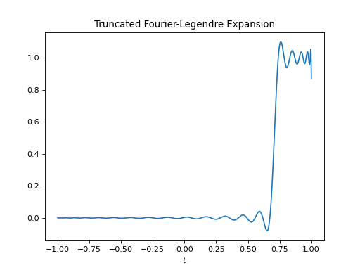
import healpy as hp
import numpy as np
from pycsphere.linop import FLT
import matplotlib.pyplot as plt

t = np.linspace(-1, 1, 4096)
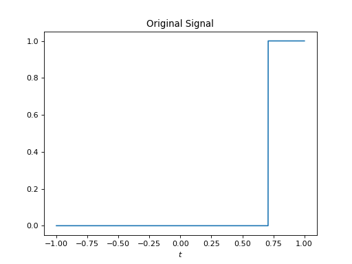
b = (np.arccos(t) <= np.pi / 4)
flt = FLT(n_max=40, t=t)
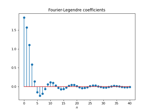
bn = flt(b)
trunc_fl_series = flt.adjoint(bn)
plt.figure()
plt.plot(t, b)
plt.xlabel('$t$')
plt.title('Original Signal')
plt.figure()
plt.stem(np.arange(flt.n_max + 1), bn)
plt.xlabel('$n$')
plt.title('Fourier-Legendre coefficients')
plt.figure()
plt.plot(t, trunc_fl_series)
plt.xlabel('$t$')
plt.title('Truncated Fourier-Legendre Expansion')
import healpy as hp
import numpy as np
from pycsphere.linop import FLT
import matplotlib.pyplot as plt

t = np.linspace(-1, 1, 4096)
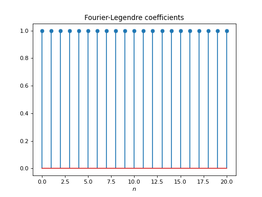
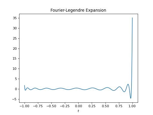
bn = np.ones(21)
flt = FLT(n_max=20, t=t)
b = flt.adjoint(bn)
plt.figure()
plt.stem(np.arange(flt.n_max + 1), bn)
plt.xlabel('$n$')
plt.title('Fourier-Legendre coefficients')
plt.figure()
plt.plot(t, b)
plt.xlabel('$t$')
plt.title('Fourier-Legendre Expansion')
Notes
Let \(\{P_{n}:[-1,1]\rightarrow\mathbb{C}, \, n\in\mathbb{N}\}\) be the Legendre polynomials. Then, any function \(b\in\mathcal{L}^2([-1, 1], \mathbb{C})\) admits a Fourier-Legendre expansion given by
\[b(t)\stackrel{a.e.}{=}\sum_{n=0}^{+\infty} \hat{b}_n\,\frac{2n+1}{4\pi} P_{n}(t),\]where the Fourier-Legendre coefficients are given by the Fourier-Legendre transform
\[\hat{b}_n:=2\pi \int_{-1}^1 b(t) P_{n}(t) \,dt, \quad n\geq 0.\]This implementation of the Fourier-Legendre transform leverages a recurrence relationship for computing efficiently Legendre polynomials, and a trapezoidal rule for approximating the integral.
Warning
Using this function with
n_maxsmaller than the function’s bandwidth may result in aliasing/smoothing artefacts.See also
-
classmethod
nmax2t(n_max: int, oversampling: float = 10.0) → numpy.ndarray[source]¶ Generate suitable samples
tfor a givenn_max.
-
classmethod
-
FLT
