Zonal Green Kernels¶

Module: pycsphere.green

Common zonal green kernels (see Chapter 4 of [FuncSphere] for a survey).

Abstract Classes

`TruncatedFourierLegendreSeries`(fn)	Truncated Fourier-Legendre series.
`ZonalGreenFunction`([order, rtol, cutoff])	Base class for zonal green functions.
`Radial2Zonal`(radial_green[, order, rtol, cutoff])	Transforms a radial Green function into a zonal Green kernel.
`ZonalGreenExponentiated`(base_green_kernel, …)	Exponentiated zonal Green kernel.

Implicit Zonal Green Kernels

`ZonalGreenSobolev`(alpha, exponent[, rtol, …])	Zonal Green kernel of the Sobolev operator \((\alpha^2\mbox{Id} -\Delta_{\mathbb{S}^2})^{\beta/2}\).
`ZonalGreenFractionalLaplaceBeltrami`(exponent)	Zonal Green kernel of the Fractional Laplace-Beltrami operator \((-\Delta_{\mathbb{S}^2})^{\beta/2}\).
`ZonalGreenIteratedLaplaceBeltrami`(exponent)	Zonal Green kernel of the iterated Laplace-Beltrami operator \(\Delta_{\mathbb{S}^2}^{k}\).
`ZonalGreenBeltrami`(k[, rtol, cutoff])	Zonal Green kernel of the Beltrami operator \(\partial_k=k(k+1)\mbox{Id}+\Delta_{\mathbb{S}^2}\).
`ZonalGreenIteratedBeltrami`(k[, rtol, cutoff])	Zonal Green kernel of the Beltrami operator \(\partial_{0\cdots k}=\partial_0\cdots\partial_k\).

Explicit Zonal Green Kernels

`ZonalMatern`(k[, epsilon, rtol, cutoff])	Matern zonal Green kernel.
`ZonalWendland`(k[, epsilon, rtol, cutoff])	Wendland zonal Green kernel.

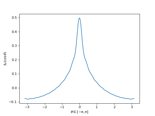
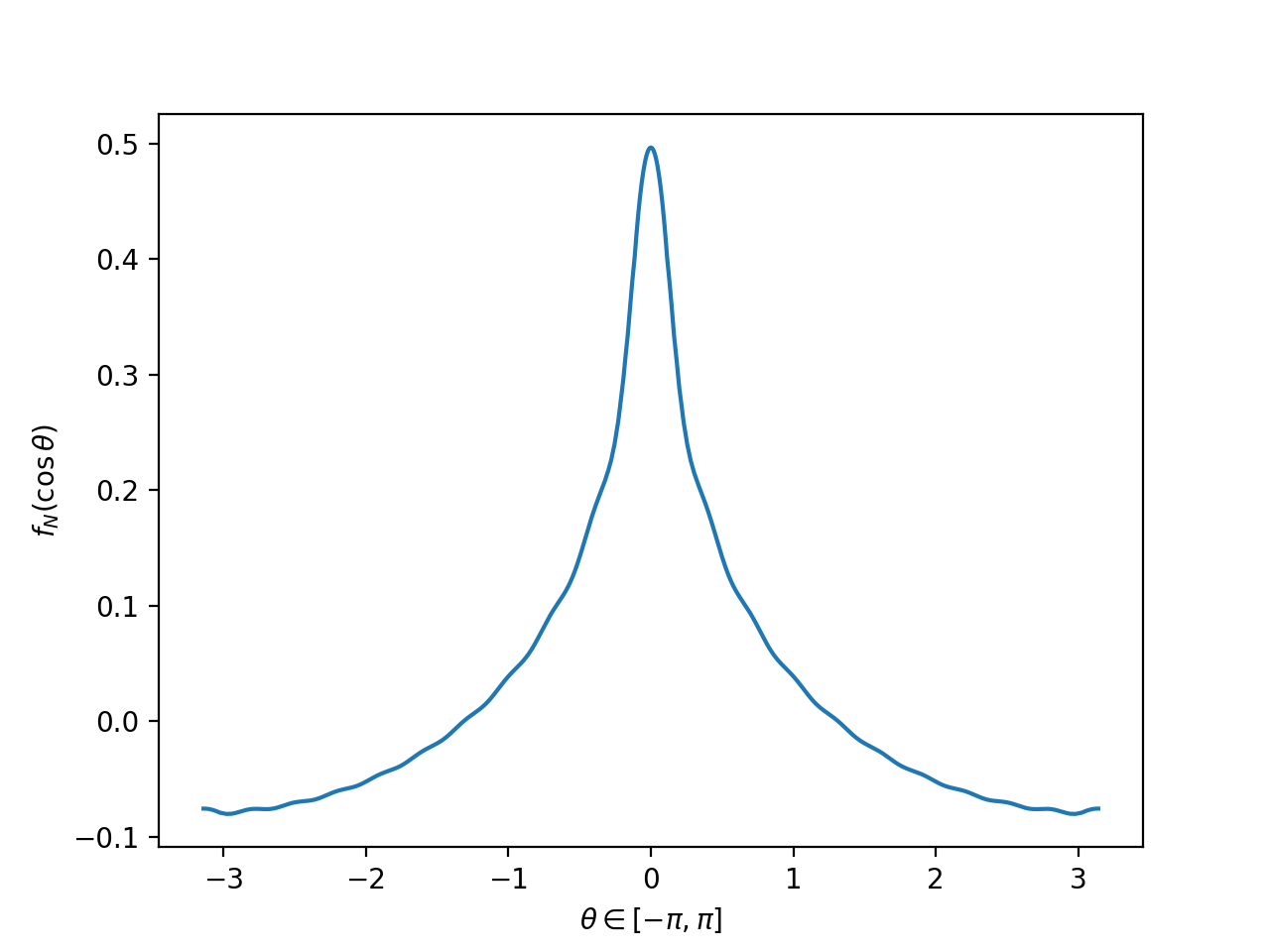
class TruncatedFourierLegendreSeries(fn: numpy.ndarray)[source]¶

Bases: object

Truncated Fourier-Legendre series.

Given coefficients \(\{\hat{f}_n, n=0,\ldots, N\}\), compute the truncated Fourier-Legendre series:

\[f_N(t):=\sum_{n=0}^N \hat{f}_n \frac{2n+1}{4\pi} P_n(t), \quad \forall t\in [-1,1].\]

Examples

import numpy as np
from pycsphere.green import TruncatedFourierLegendreSeries

n_max=20
n=np.arange(0, n_max + 1).astype(np.float)
fn=0*n; fn[n>0]=(n[n>0]*(n[n>0]+1))**(-1)
fN=TruncatedFourierLegendreSeries(fn)
theta=np.linspace(-np.pi, np.pi, 1024)
plt.plot(theta, fN(np.cos(theta)))
plt.ylabel('$f_N(\\cos\\theta)$')
plt.xlabel('$\\theta\\in[-\\pi,\\pi]$')

(Source code, png, hires.png, pdf)

Notes

The TruncatedFourierLegendreSeries is computed by interpolating linearly the result of FourierLegendreTransform.

__init__(fn: numpy.ndarray)[source]¶

Parameters: fn (np.ndarray) – Fourier-Legendre coefficients.

class ZonalGreenFunction(order: Optional[float] = None, rtol: float = 0.0001, cutoff: Optional[int] = None)[source]¶

Bases: abc.ABC

Base class for zonal green functions.

Any subclass/instance of this class must implement the abstract method _compute_fl_coefficients.

Notes

Consider a spherical pseudpo-differential operator acting on a spherical function \(h(\mathbf{r})\) as:

\[\mathcal{D} h:=\sum_{n=0}^{+\infty}\hat{D}_n \left[\sum_{m=-n}^{n}\hat{h}_n^m Y_n^m\right],\]

where \(\{\hat{D}_n\}_{n\in\mathbb{N}}\in\mathbb{R}^\mathbb{N}\) is a sequence of real numbers such that the set

\[\mathcal{K}_\mathcal{D}:=\left\{n\in\mathbb{N}:\; \vert \hat{D}_n\vert=0\right\},\]

is finite and

\[\vert\hat{D}_n\vert=\Theta\left(n^p\right),\]

for some real number \(p\geq 0\), called the spectral growth order of \(\mathcal{D}\). Then, the zonal Green kernel of \(\mathcal{D}\) is given by Proposition 4 of [FuncSphere]:

\[\psi_{\mathcal{D}}(\langle\mathbf{r}, \mathbf{s}\rangle) := \sum_{{n\in\mathbb{N}\backslash\mathcal{K}_\mathcal{D}}} \frac{2n+1}{4\pi \hat{D}_n}P_{n}(\langle\mathbf{r}, \mathbf{s}\rangle),\quad \mathbf{r}\in\mathbb{S}^{2},\]

where \(P_{n}\) are the Legendre polynomials. The summation above is truncated to a large enough \(N\) called the effective bandwidth of the zonal Green kernel.

__init__(order: Optional[float] = None, rtol: float = 0.0001, cutoff: Optional[int] = None)[source]¶

Parameters

order (Optional[float]) – Spectral growth order of the associated pseudo-differential operator.
rtol (float) – Threshold for defining the effective bandwidth of the zonal Green kernel.
cutoff (Optional[int]) – Effective bandwidth of the zonal Green kernel.

get_cutoff(min_cutoff: int = 16) → int[source]¶

Compute the effective bandwidth of the zonal Green kernel.

Parameters: min_cutoff (int) – Minimal bandwidth.
Returns: Effective bandwidth of the zonal Green kernel.
Return type: int

green_kernel() → Callable[source]¶

Compute the zonal Green kernel.

Returns: The zonal Green kernel as a callable function.
Return type: Callable

plot(resolution: int = 1024, color: str = None, linewidth: Union[int, float] = 2, angles: bool = False, fraction: float = 1, fhandle: Optional[Any] = None)[source]¶

Plot the zonal Green kernel.

Parameters

resolution (int) – Resolution of the uniform grid on which the Green kernel is sampled.
color (str) – Color of the line.
linewidth (Union[int, float]) – Line width.
angles (bool) – If True plot \(\psi(\cos(\theta))\), otherwise plot \(\psi(t)\).
fraction (float) – Plot over [-fraction, fraction] (if angles==False) or [-np.pi*fraction, np.pi*fraction] (if angles==True) with 0<fraction<=1.
fhandle (Optional[Any]) – Figure handle in which to plot.

spectrum(n_max=None, cast: Callable = <function real>, fhandle: Optional[Any] = None, color_index: int = 0)[source]¶: Plot the Fourier-Legendre spectrum.

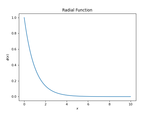
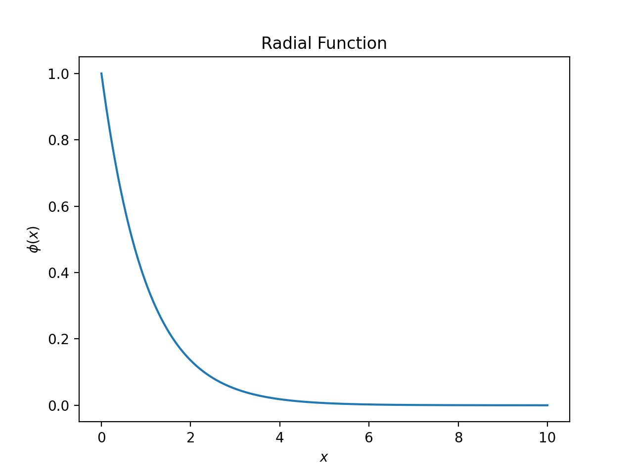
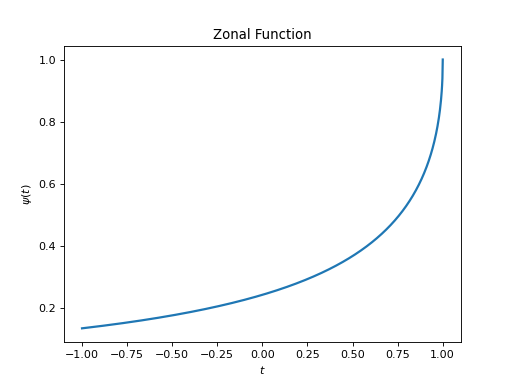
class Radial2Zonal(radial_green: Callable, order: Optional[float] = None, rtol: float = 0.0001, cutoff: Optional[int] = None)[source]¶

Bases: pycsphere.green.ZonalGreenFunction

Transforms a radial Green function into a zonal Green kernel.

Let \(\phi:\mathbb{R}_+\to \mathbb{C}\) be a radial function. The zonal Green kernel associated to \(\phi\) is defined as:

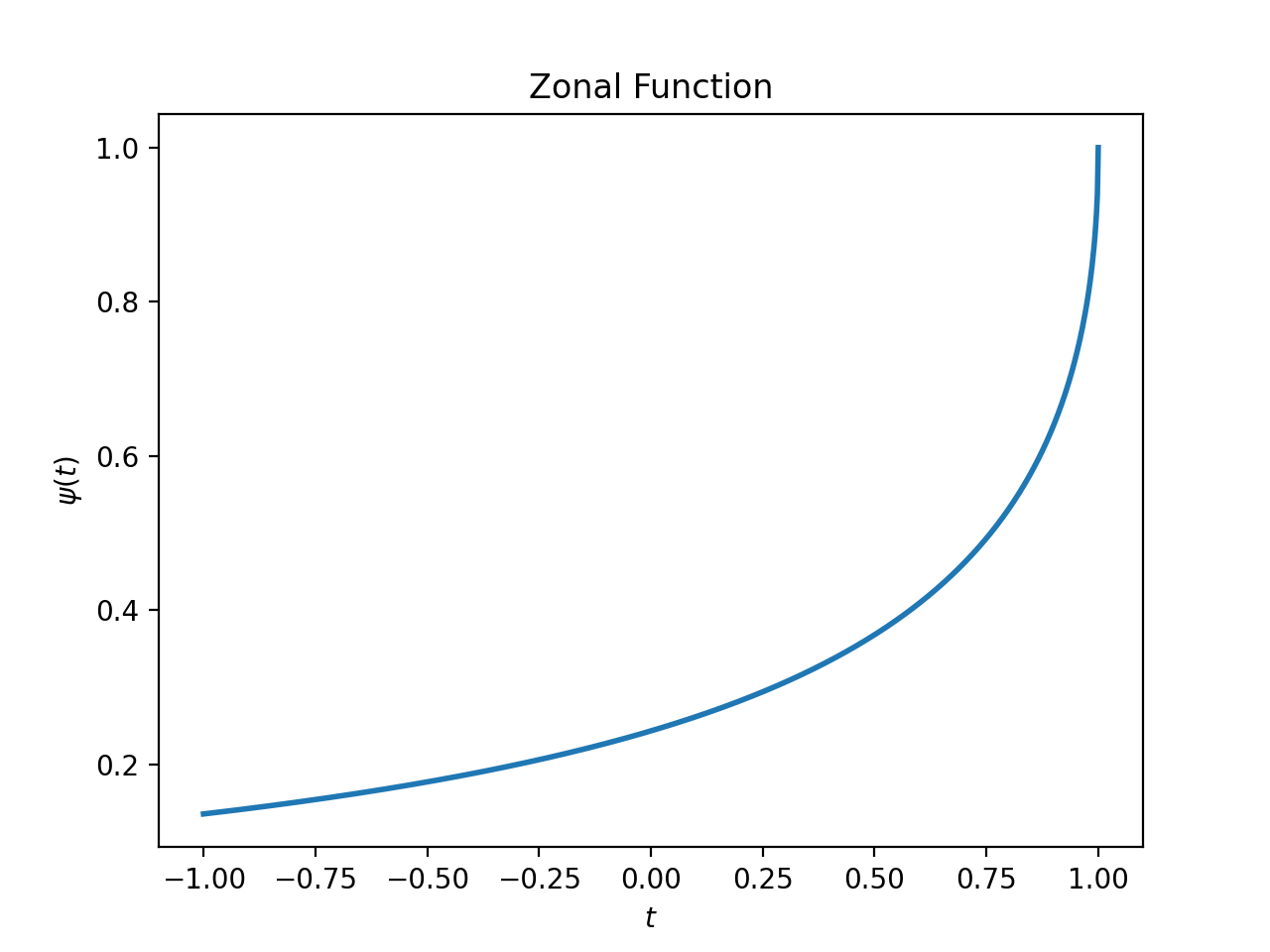
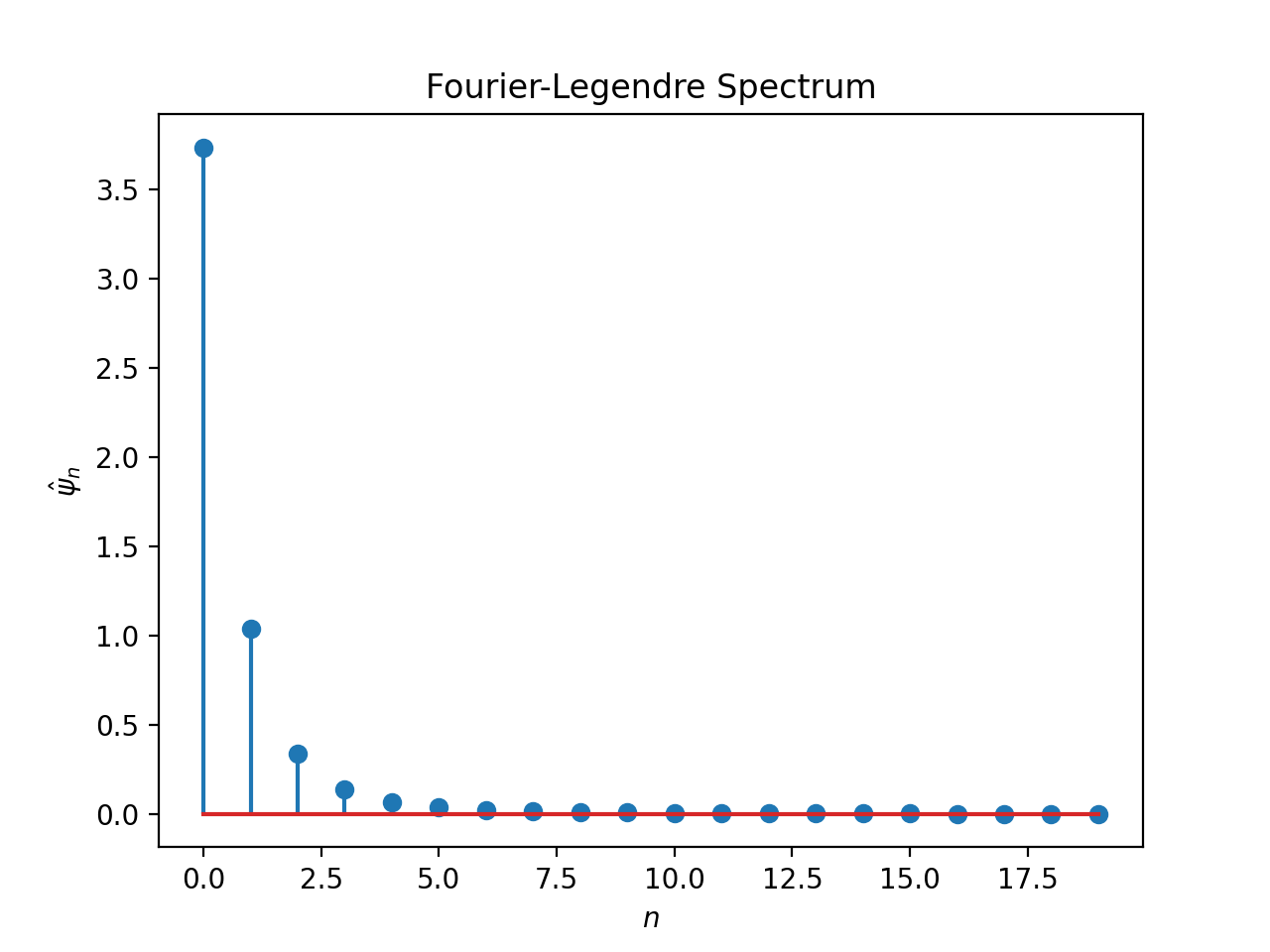
\[\psi(t):=\phi(\sqrt{2-2t}), \qquad t\in [-1,1].\]

Examples

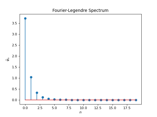
from pycsphere.green import Radial2Zonal
from pycsou.math import Matern

radial_green=Matern(k=0, epsilon=1)
zonal_green=Radial2Zonal(radial_green=radial_green, order=3 / 2)
plt.plot(np.linspace(0,10,1024), radial_green(np.linspace(0,10,1024)))
plt.xlabel('$x$')
plt.ylabel('$\\phi(x)$')
plt.title('Radial Function')
zonal_green.plot()
zonal_green.spectrum(n_max=20)

(Source code)

(png, hires.png, pdf)¶

(png, hires.png, pdf)¶

(png, hires.png, pdf)¶

__init__(radial_green: Callable, order: Optional[float] = None, rtol: float = 0.0001, cutoff: Optional[int] = None)[source]¶

Parameters

radial_green (Callable) – Radial green function (must have a method __call__ for evaluation).
order (Optional[float]) – Spectral growth order of the associated pseudo-differential operator.
rtol (float) – Threshold for defining the effective bandwidth of the zonal Green kernel.
cutoff (Optional[int]) – Effective bandwidth of the zonal Green kernel.

green_kernel()[source]¶

Compute the zonal Green kernel.

Returns: The zonal Green kernel as a callable function.
Return type: Callable

class ZonalGreenExponentiated(base_green_kernel: pycsphere.green.ZonalGreenFunction, exponent: int, rtol: float = 0.0001, cutoff: Optional[int] = None)[source]¶

Bases: pycsphere.green.ZonalGreenFunction

Exponentiated zonal Green kernel.

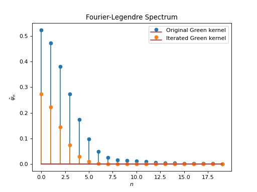
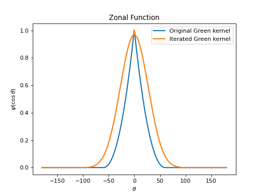
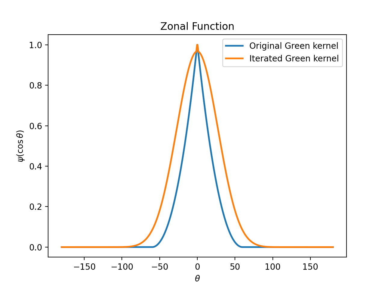
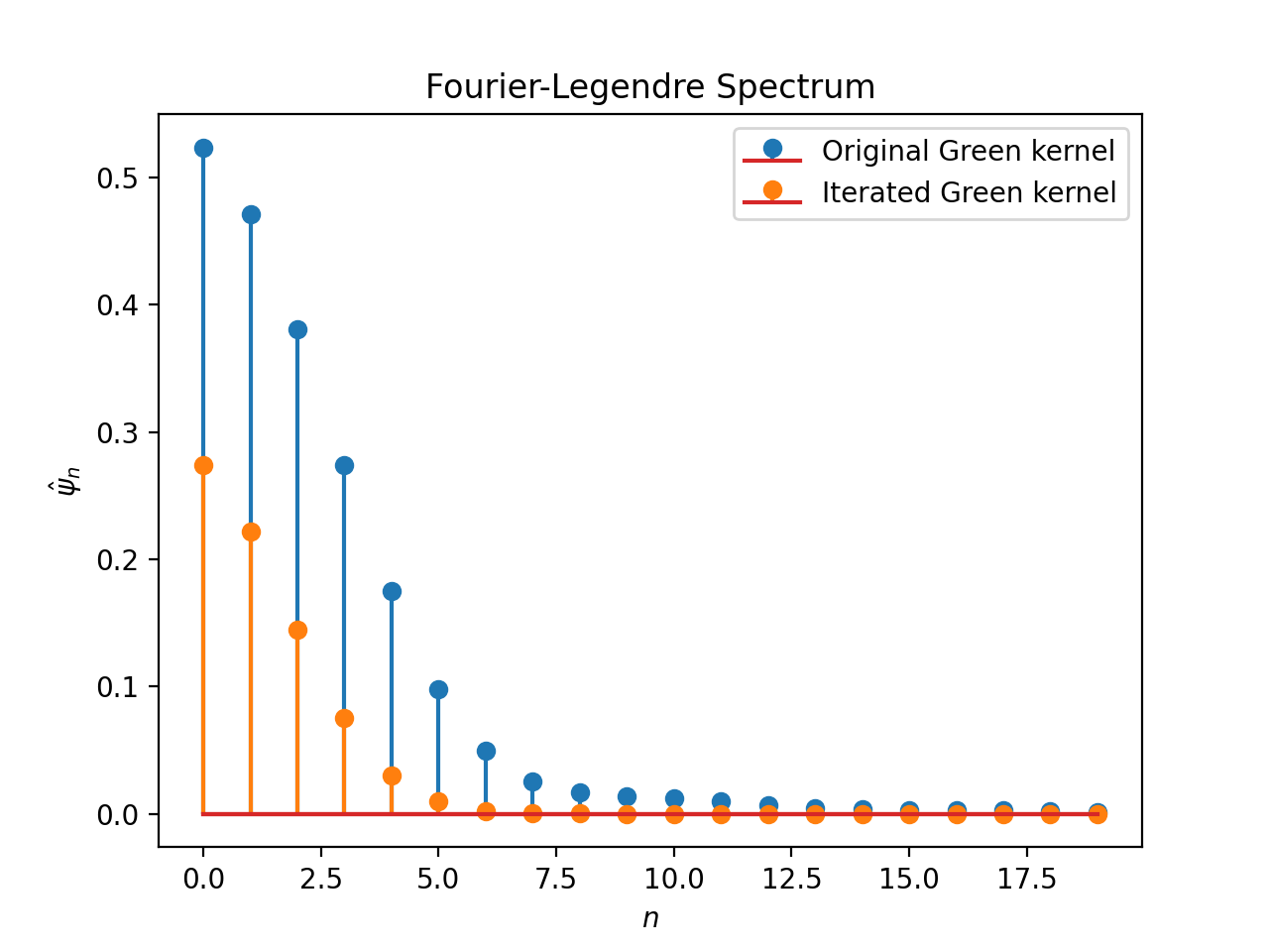
Consider a zonal Green kernel \(\psi:[-1,1]\to \mathbb{C}\) with Fourier-Legendre expansion:

\[\psi(t)=\sum_{n=0}^{+\infty}\frac{2n+1}{4\pi\hat{D}_n} P_n(t), \quad t\in[-1,1].\]

Then, the exponentiated zonal Green kernel \(\psi^{(\alpha)}:[-1,1]\to \mathbb{C}, \; \alpha\in\mathbb{R}_+\) has Fourier-Legendre expansion:

\[\psi^{(\alpha)}(t)=\sum_{n=0}^{+\infty}\frac{2n+1}{4\pi\hat{D}^\alpha_n} P_n(t), \quad t\in[-1,1].\]

Examples

from pycsphere.green import ZonalWendland, ZonalGreenExponentiated

zonal_green=ZonalWendland(k=0)
iterated_zonal_green=ZonalGreenExponentiated(zonal_green, exponent=2)
zonal_green.plot(angles=True, fhandle=1)
iterated_zonal_green.plot(angles=True, fhandle=1)
plt.legend(['Original Green kernel', 'Iterated Green kernel'])
zonal_green.spectrum(n_max=20, fhandle=2, color_index=0)
iterated_zonal_green.spectrum(n_max=20, fhandle=2, color_index=1)
plt.legend(['Original Green kernel', 'Iterated Green kernel'])

(Source code)

(png, hires.png, pdf)¶

(png, hires.png, pdf)¶

__init__(base_green_kernel: pycsphere.green.ZonalGreenFunction, exponent: int, rtol: float = 0.0001, cutoff: Optional[int] = None)[source]¶

Parameters

base_green_kernel (ZonalGreenFunction) – Zonal Green kernel to be exponentiated.
exponent (int) – Exponent \(\alpha>0\).
rtol (float) – Threshold for defining the effective bandwidth of the zonal Green kernel.
cutoff (Optional[int]) – Effective bandwidth of the zonal Green kernel.

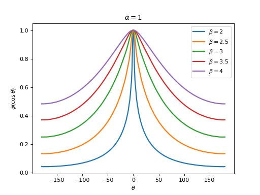
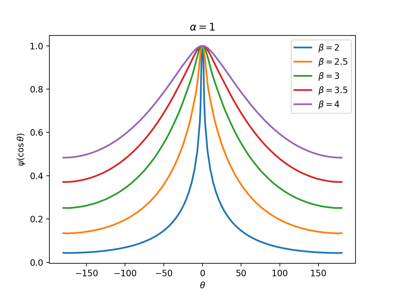
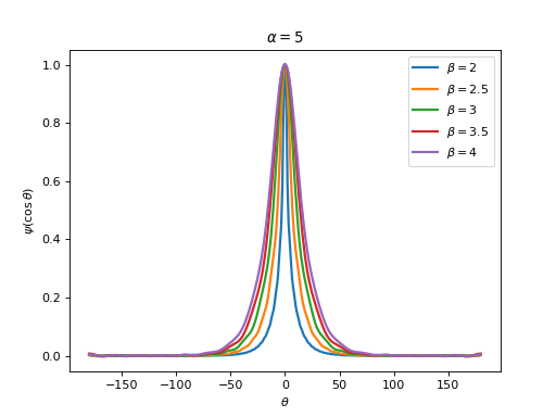
class ZonalGreenSobolev(alpha: Union[float, int], exponent: Union[int, float], rtol: float = 0.0001, cutoff: Optional[int] = None)[source]¶

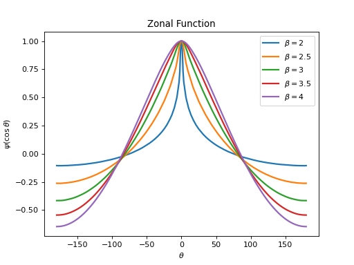
Bases: pycsphere.green.ZonalGreenFunction

Zonal Green kernel of the Sobolev operator \((\alpha^2\mbox{Id} -\Delta_{\mathbb{S}^2})^{\beta/2}\).

Examples

from pycsphere.green import ZonalGreenSobolev

for exp in [2,2.5,3,3.5,4]:
    zonal_green=ZonalGreenSobolev(alpha=1., exponent=exp)
    zonal_green.plot(angles=True, fhandle=1)
plt.legend([f'$\\beta={np.round(val, 1)}$' for val in [2,2.5,3,3.5,4]])
plt.title('$\\alpha=1$')

for exp in [2,2.5,3,3.5,4]:
    zonal_green=ZonalGreenSobolev(alpha=5., exponent=exp)
    zonal_green.plot(angles=True, fhandle=2)
plt.legend([f'$\\beta={np.round(val, 1)}$' for val in [2,2.5,3,3.5,4]])
plt.title('$\\alpha=5$')

(Source code)

(png, hires.png, pdf)¶

(png, hires.png, pdf)¶

Notes

We have in this case \(\hat{D}_n=(\alpha^2+n(n+1))^{\beta/2},\) \(\hat{D}_n>0\), \(|\hat{D}_n|=\Theta(n^{\beta})\), and \(\mathcal{K}_{\mathcal{D}}=\emptyset\).

__init__(alpha: Union[float, int], exponent: Union[int, float], rtol: float = 0.0001, cutoff: Optional[int] = None)[source]¶

Parameters

alpha (Union[complex, float, int]) – Parameter \(\alpha\in\mathbb{R}\). Large values of \(\alpha\) yield more localised Green kernels.
exponent (Union[int, float]) – Exponent \(\beta\geq 1.\)
rtol (float) – Threshold for defining the effective bandwidth of the zonal Green kernel.
cutoff (Optional[int]) – Effective bandwidth of the zonal Green kernel.

class ZonalGreenFractionalLaplaceBeltrami(exponent: float, rtol: float = 0.0001, cutoff: Optional[int] = None)[source]¶

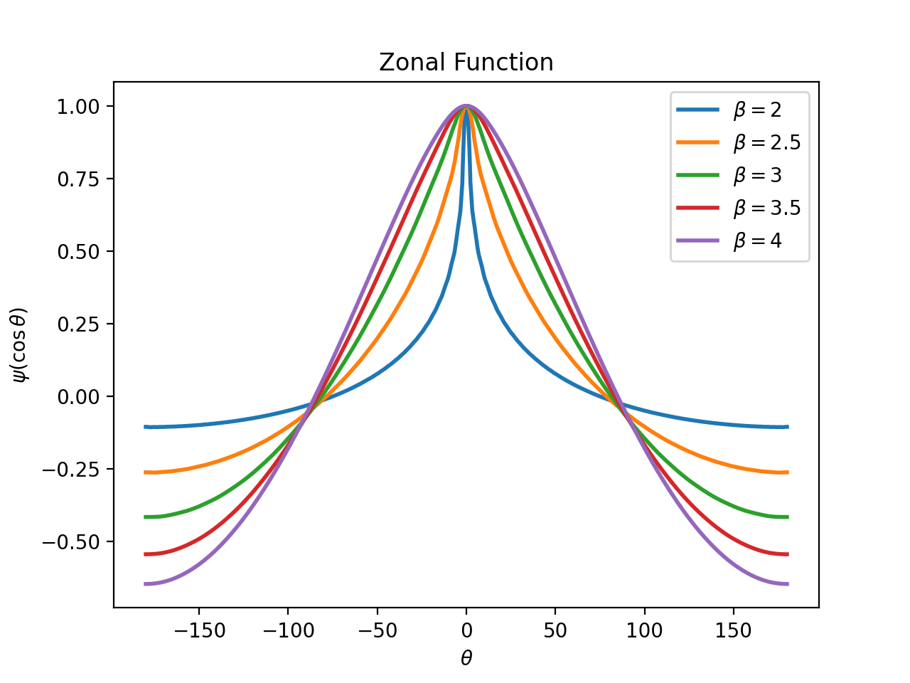
Bases: pycsphere.green.ZonalGreenSobolev

Zonal Green kernel of the Fractional Laplace-Beltrami operator \((-\Delta_{\mathbb{S}^2})^{\beta/2}\).

Examples

from pycsphere.green import ZonalGreenFractionalLaplaceBeltrami

for exp in [2,2.5,3,3.5,4]:
    zonal_green=ZonalGreenFractionalLaplaceBeltrami(exponent=exp)
    zonal_green.plot(angles=True, fhandle=1)
plt.legend([f'$\\beta={np.round(val, 1)}$' for val in [2,2.5,3,3.5,4]])

(Source code, png, hires.png, pdf)

Notes

We have in this case \(\hat{D}_n=(n(n+1))^{\beta/2},\) \(\hat{D}_n\geq 0\), \(|\hat{D}_n|=\Theta(n^{\beta})\), and \(\mathcal{K}_{\mathcal{D}}=\{0\}\). See Example 4.2 of [FuncSphere] for a closed-form formula of the zonal Green kernel for \(\beta=4\). The case \(\beta=1\) yields the square-root of the Laplace-Beltrami operator, which is intimately linked to the spherical divergence and gradient differential operators.

See also

ZonalGreenIteratedLaplaceBeltrami

__init__(exponent: float, rtol: float = 0.0001, cutoff: Optional[int] = None)[source]¶

Parameters

exponent (Union[int, float]) – Exponent \(\beta\geq 1.\)
rtol (float) – Threshold for defining the effective bandwidth of the zonal Green kernel.
cutoff (Optional[int]) – Effective bandwidth of the zonal Green kernel.

class ZonalGreenIteratedLaplaceBeltrami(exponent: int, rtol: float = 0.0001, cutoff: Optional[int] = None)[source]¶

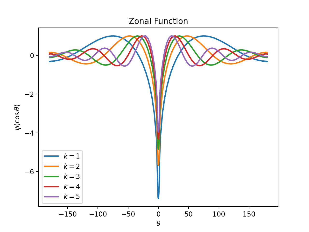
Bases: pycsphere.green.ZonalGreenFunction

Zonal Green kernel of the iterated Laplace-Beltrami operator \(\Delta_{\mathbb{S}^2}^{k}\).

Examples

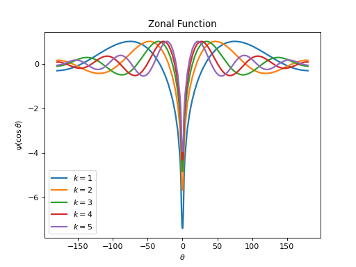
from pycsphere.green import ZonalGreenIteratedLaplaceBeltrami

for exp in [1,2,3,4,5]:
    zonal_green=ZonalGreenIteratedLaplaceBeltrami(exponent=exp)
    zonal_green.plot(angles=True, fhandle=1)
plt.legend([f'$k={np.round(val, 1)}$' for val in [1,2,3,4,5]])

(Source code, png, hires.png, pdf)

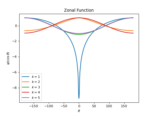
Notes

We have in this case \(\hat{D}_n=(-n(n+1))^{k},\) \(\hat{D}_n\in \mathbb{R}\), \(|\hat{D}_n|=\Theta(n^{2k})\), and \(\mathcal{K}_{\mathcal{D}}=\{0\}\). See Example 4.2 of [FuncSphere] for a closed-form formula of the zonal Green kernel for \(k=2\).

See also

ZonalGreenFractionalLaplaceBeltrami

__init__(exponent: int, rtol: float = 0.0001, cutoff: Optional[int] = None)[source]¶

Parameters

exponent (int) – Exponent \(k\geq 1.\)
rtol (float) – Threshold for defining the effective bandwidth of the zonal Green kernel.
cutoff (Optional[int]) – Effective bandwidth of the zonal Green kernel.

class ZonalGreenBeltrami(k: int, rtol: float = 0.0001, cutoff: Optional[int] = None)[source]¶

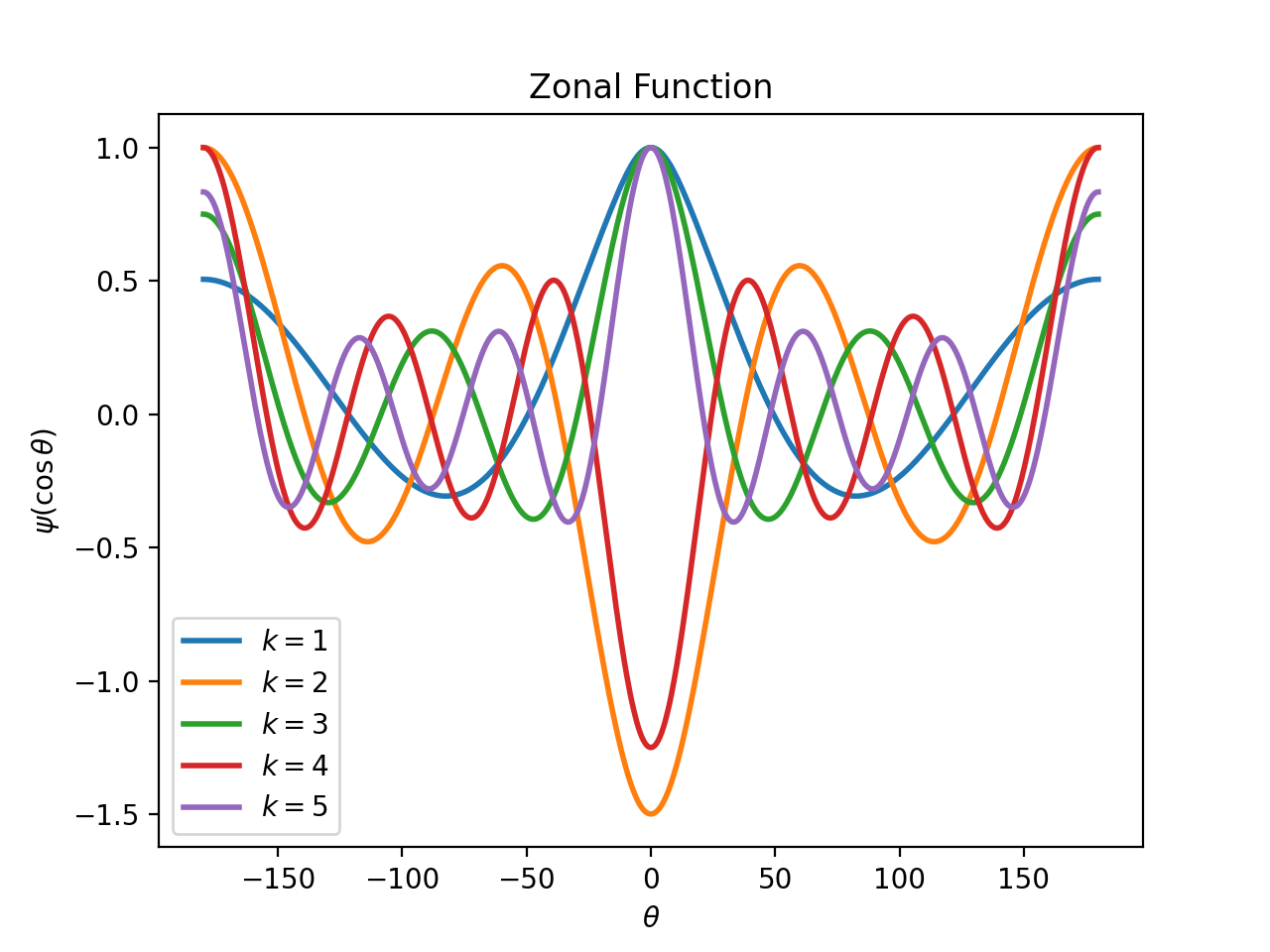
Bases: pycsphere.green.ZonalGreenFunction

Zonal Green kernel of the Beltrami operator \(\partial_k=k(k+1)\mbox{Id}+\Delta_{\mathbb{S}^2}\).

Examples

from pycsphere.green import ZonalGreenBeltrami

for k in [1,2,3,4,5]:
    zonal_green=ZonalGreenBeltrami(k=k)
    zonal_green.plot(angles=True, fhandle=1)
plt.legend([f'$k={np.round(val, 1)}$' for val in [1,2,3,4,5]])

(Source code, png, hires.png, pdf)

Notes

We have in this case \(\hat{D}_n=k(k+1)-n(n+1),\) \(\hat{D}_n\in \mathbb{R}\), \(|\hat{D}_n|=\Theta(n^{2})\), and \(\mathcal{K}_{\mathcal{D}}=\{k\}\). See Chapter 4 of [FuncSphere] for properties of Beltrami operators.

See also

ZonalGreenIteratedBeltrami

__init__(k: int, rtol: float = 0.0001, cutoff: Optional[int] = None)[source]¶

Parameters

k (int) – Parameter \(k\geq 1.\)
rtol (float) – Threshold for defining the effective bandwidth of the zonal Green kernel.
cutoff (Optional[int]) – Effective bandwidth of the zonal Green kernel.

class ZonalGreenIteratedBeltrami(k: int, rtol: float = 0.0001, cutoff: Optional[int] = None)[source]¶

Bases: pycsphere.green.ZonalGreenFunction

Zonal Green kernel of the Beltrami operator \(\partial_{0\cdots k}=\partial_0\cdots\partial_k\).

Examples

from pycsphere.green import ZonalGreenIteratedBeltrami

for k in [1,2,3,4,5]:
    zonal_green=ZonalGreenIteratedBeltrami(k=k)
    zonal_green.plot(angles=True, fhandle=1)
plt.legend([f'$k={np.round(val, 1)}$' for val in [1,2,3,4,5]])

(Source code, png, hires.png, pdf)

Notes

We have in this case \(\hat{D}_n=\Pi_{j=0}^k j(j+1)-n(n+1),\) \(\hat{D}_n\in \mathbb{R}\), \(|\hat{D}_n|=\Theta(n^{2(k+1)})\), and \(\mathcal{K}_{\mathcal{D}}=\{0,\ldots,k\}\). See Chapter 4 of [FuncSphere] for properties of Beltrami operators.

See also

ZonalGreenBeltrami

__init__(k: int, rtol: float = 0.0001, cutoff: Optional[int] = None)[source]¶

Parameters

k (int) – Parameter \(k\geq 1.\)
rtol (float) – Threshold for defining the effective bandwidth of the zonal Green kernel.
cutoff (Optional[int]) – Effective bandwidth of the zonal Green kernel.

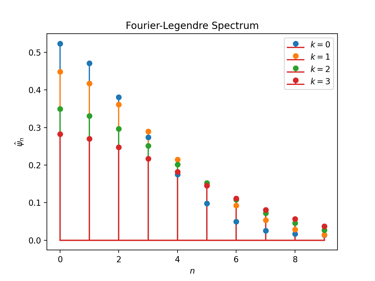
class ZonalMatern(k: int, epsilon: float = 1.0, rtol: float = 0.0001, cutoff: Optional[int] = None)[source]¶

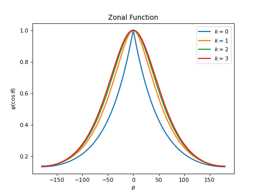
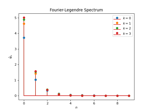
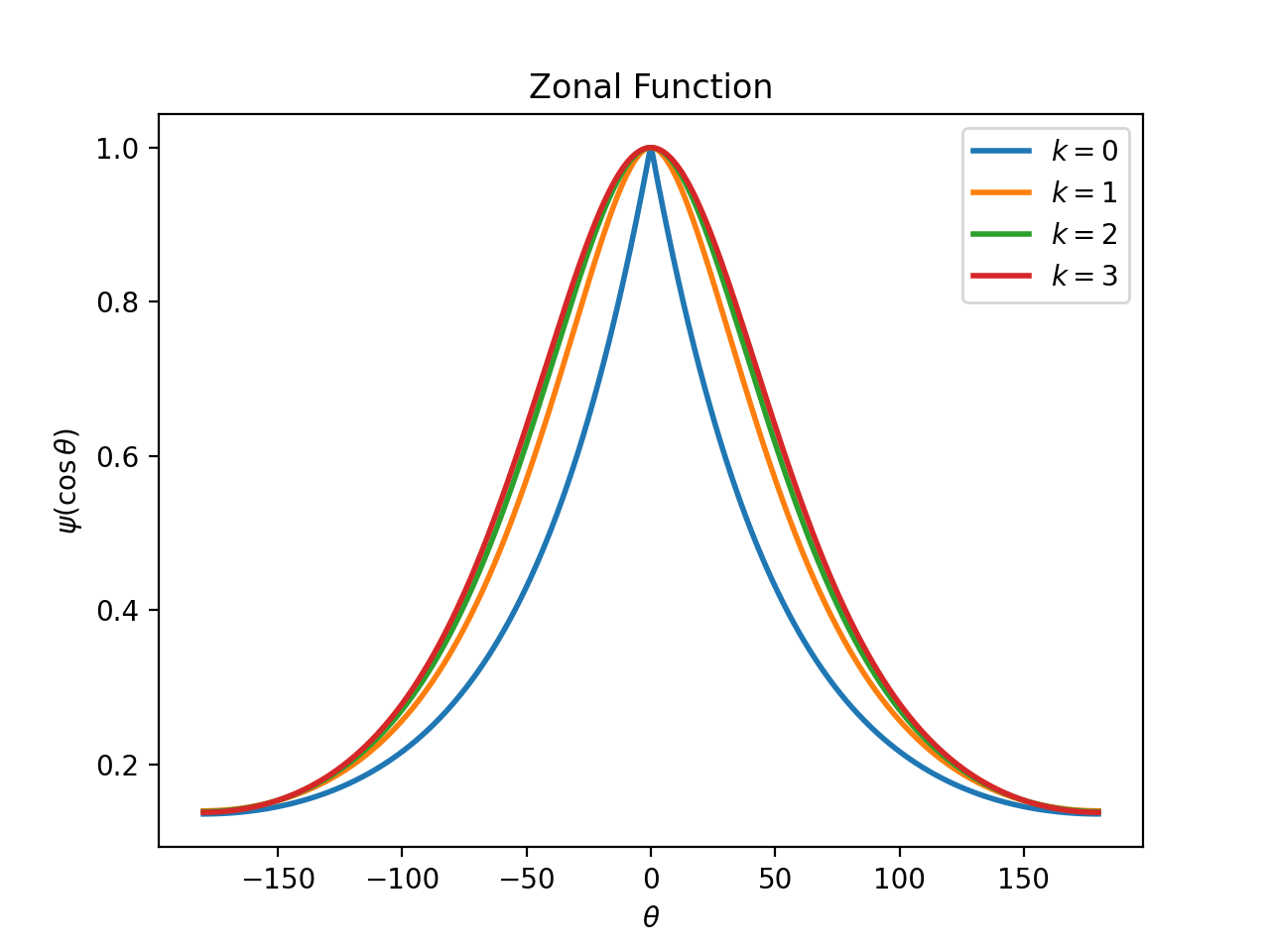
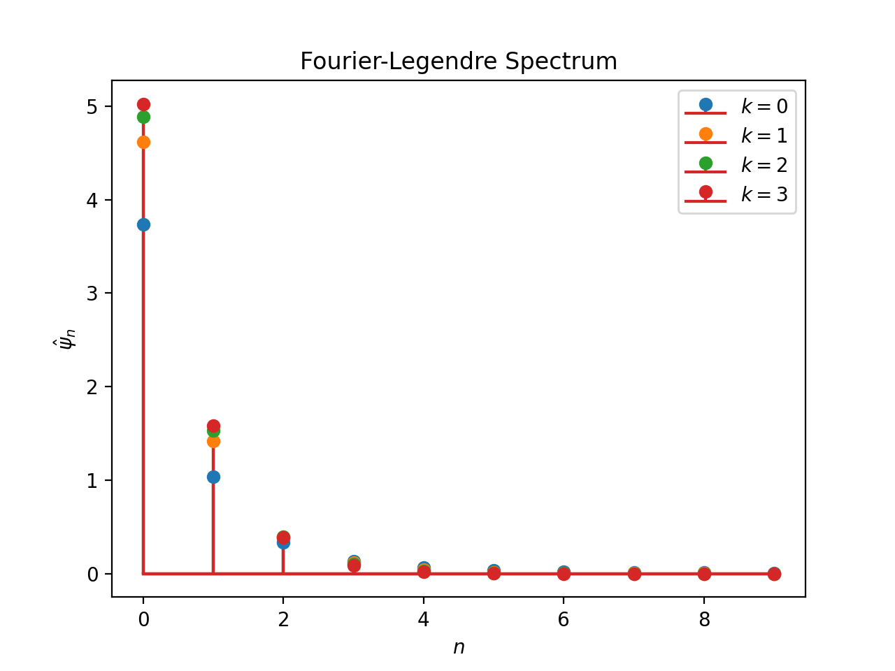
Bases: pycsphere.green.Radial2Zonal

Matern zonal Green kernel.

The Matern zonal Green kernel is obtained by restricting the radial Matern function pycsou.math.green.Matern to the sphere as described in pycsphere.green.Radial2Zonal.

Examples

from pycsphere.green import ZonalMatern

for k in [0, 1,2,3]:
    zonal_green=ZonalMatern(k=k)
    zonal_green.plot(angles=True, fhandle=1)
plt.legend([f'$k={np.round(val, 1)}$' for val in [0, 1,2,3]])

for k in [0, 1,2,3]:
    zonal_green=ZonalMatern(k=k)
    zonal_green.spectrum(n_max=10, fhandle=2, color_index=k)
plt.legend([f'$k={np.round(val, 1)}$' for val in [0, 1,2,3]])

(Source code)

(png, hires.png, pdf)¶

(png, hires.png, pdf)¶

Notes

See Chapter 8 of [FuncSphere] for definitions, closed-form formulas and properties.

See also

pycsou.math.green.Matern, Wendland

__init__(k: int, epsilon: float = 1.0, rtol: float = 0.0001, cutoff: Optional[int] = None)[source]¶

Parameters

k (int, [0, 1 ,2 ,3]) – Order of the Matern function.
epsilon (float) – Spread of the Matern function.
rtol (float) – Threshold for defining the effective bandwidth of the zonal Green kernel.
cutoff (Optional[int]) – Effective bandwidth of the zonal Green kernel.

Notes

See the help of pycsou.math.green.Matern for more details on the parameters k and epsilon.

class ZonalWendland(k: int, epsilon: float = 1.0, rtol: float = 0.0001, cutoff: Optional[int] = None)[source]¶

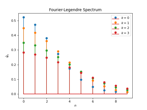
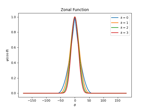
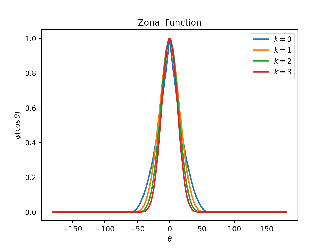
Bases: pycsphere.green.Radial2Zonal

Wendland zonal Green kernel.

The Wendland zonal Green kernel is obtained by restricting the radial Wendland function pycsou.math.green.Wendland to the sphere as described in pycsphere.green.Radial2Zonal.

Examples

from pycsphere.green import ZonalWendland

for k in [0, 1,2,3]:
    zonal_green=ZonalWendland(k=k)
    zonal_green.plot(angles=True, fhandle=1)
plt.legend([f'$k={np.round(val, 1)}$' for val in [0, 1,2,3]])

for k in [0, 1,2,3]:
    zonal_green=ZonalWendland(k=k)
    zonal_green.spectrum(n_max=10, fhandle=2, color_index=k)
plt.legend([f'$k={np.round(val, 1)}$' for val in [0, 1,2,3]])

(Source code)

(png, hires.png, pdf)¶

(png, hires.png, pdf)¶

Notes

See Chapter 8 of [FuncSphere] for definitions, closed-form formulas and properties.

See also

pycsou.math.green.Wendland, Matern

__init__(k: int, epsilon: float = 1.0, rtol: float = 0.0001, cutoff: Optional[int] = None)[source]¶

Parameters

k (int, [0, 1 ,2 ,3]) – Order of the Wendland function.
epsilon (float) – Spread of the Wendland function.
rtol (float) – Threshold for defining the effective bandwidth of the zonal Green kernel.
cutoff (Optional[int]) – Effective bandwidth of the zonal Green kernel.

Notes

See the help of pycsou.math.green.Wendland for more details on the parameters k and epsilon.