Green Functions

Module: pycsou.math.green

Green functions of common pseudo-differential operators.

Classes

CausalGreenExponential(k[, alpha])	Causal Green function of \((D+\alpha\mbox{Id})^k\).
CausalGreenIteratedDerivative(k)	Causal Green function of the iterated derivative \(D^k\).
Matern(k[, epsilon])	Matern function for \(k\in\{0,1,2,3\}\).
SubGaussian(alpha[, epsilon])	Sub-Gaussian function.
Wendland(k[, epsilon])	Wendland functions for \(k\in\{0, 1, 2, 3\}\).

class Matern(k: int, epsilon: float = 1.0)

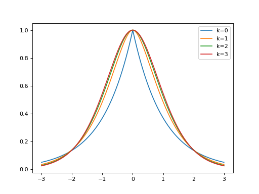
Bases: object

Matern function for \(k\in\{0,1,2,3\}\).

Examples

import matplotlib.pyplot as plt
import numpy as np
from pycsou.math.green import Matern

x=np.linspace(-3,3,1024)
for k in range(4):
   matern=Matern(k)
   plt.plot(x, matern(np.abs(x)))
plt.legend(['k=0', 'k=1', 'k=2', 'k=3'])

(Source code, png, hires.png, pdf)

Notes

The Matern function is defined in full generality as ([GaussProcesses], eq (4.14)):

\[S_\nu^\epsilon(r) = \frac{2^{1-\nu}}{\Gamma(\nu)}\left(\frac{\sqrt{2\nu} r}{\epsilon}\right)^\nu K_{\nu}\left(\frac{\sqrt{2\nu} r}{\epsilon}\right), \qquad \forall r\in\mathbb{R}_+,\]

with \(\nu, \epsilon>0\), \(\Gamma\) and \(K_\nu\) are the Gamma and modified Bessel function of the second kind, respectively. The parameter \(nu\) determines the smoothness of the Matern function (the higher, the smoother). The parameter \(epsilon\) determines the localisation of the Matern function (the higher, the more localised). For \(\nu\in\mathbb{N}+1/2\) the above equation simplifies to:

\[S_{k+1/2}^\epsilon(r)=\exp\left(-\frac{\sqrt{2\nu} r}{\epsilon}\right) \frac{k!}{(2k)!} \sum_{i=0}^{k} \frac{(k+i)!}{i!(k-i)!}\left(\frac{\sqrt{8\nu}r}{\epsilon}\right)^{k-i}, \qquad \forall r\in\mathbb{R}_+,\]

with \(k\in \mathbb{N}\). This class provides the Matern function for \(k\in\{0,1,2,3\}\) (Matern functions with \(k>3\) are nearly indistinguishable from a Gaussian function with standard deviation \(\epsilon\)). The Matern radial basis function \(S_{\nu}^\epsilon(\|\cdot\|)\) in \(\mathbb{R}^d\) is proportional to the Green function of the pseudo-differential operator \(\left(\mbox{Id} - \frac{\epsilon^2}{2\nu}\Delta_{\mathbb{R}^d}\right)^{2\nu+d}\), i.e. \(\left(\mbox{Id} - \frac{\epsilon^2}{2\nu}\Delta_{\mathbb{R}^d}\right)^{2\nu+d}S_{\nu}^\epsilon(\|\cdot\|)\propto \delta\).

See also

Wendland

__init__(k: int, epsilon: float = 1.0)

Parameters

• k (int, Literal[0, 1 ,2 ,3]) – Order of the Matern function.

• epsilon (float) – Spread of the Matern function (support is approximately 3*epsilon).

support(sigmas: int = 3) → float

Effective support of the Matern function using a Gaussian approximation.

The approximation is poor for \(k=0\).

Parameters

sigmas (int) – Number of sigmas defining the support of the approximating Gaussian function.

Returns

Approximate effective support of the Matern function.

Return type

float

class Wendland(k: int, epsilon: float = 1.0)

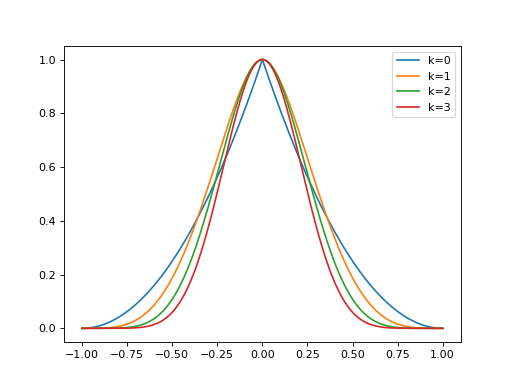
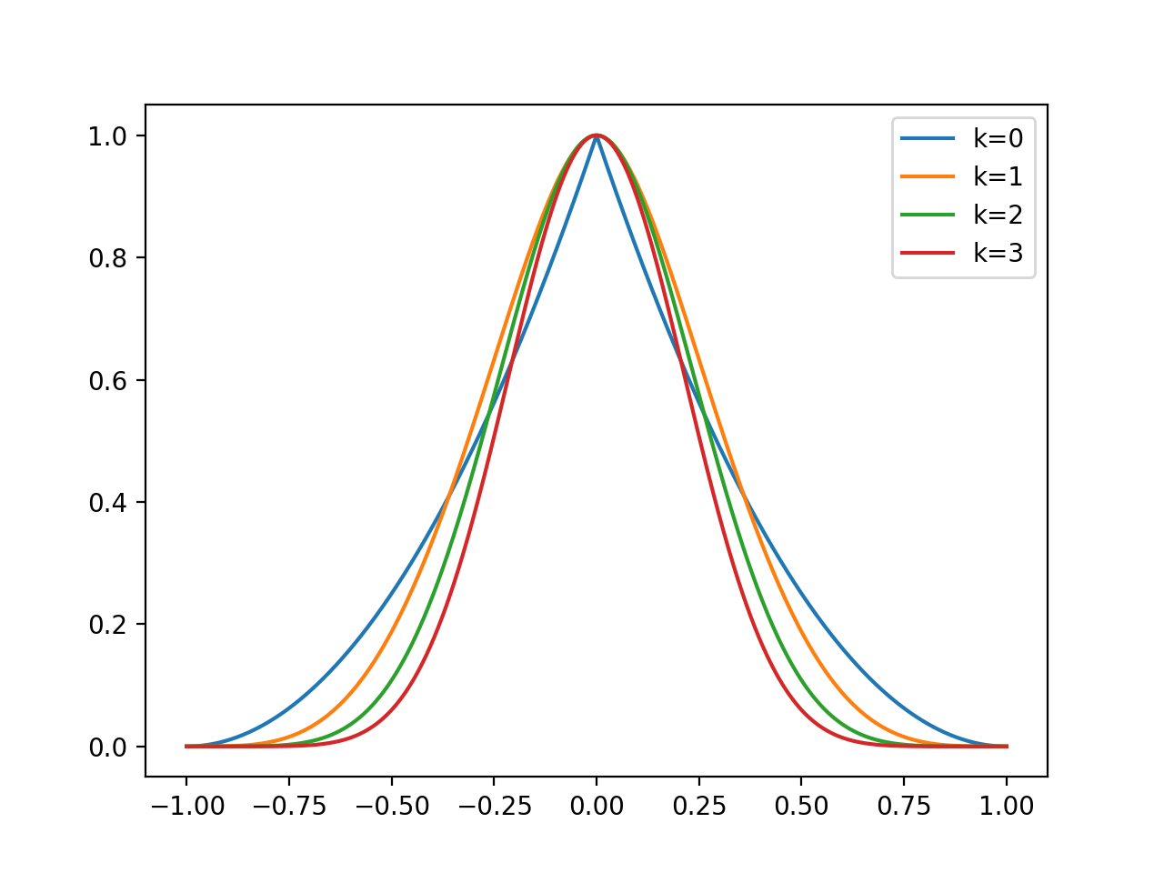
Bases: object

Wendland functions for \(k\in\{0, 1, 2, 3\}\).

Examples

import matplotlib.pyplot as plt
import numpy as np
from pycsou.math.green import Wendland

x=np.linspace(-1,1,1024)
for k in range(4):
   wendland=Wendland(k)
   plt.plot(x, wendland(np.abs(x)))
plt.legend(['k=0', 'k=1', 'k=2', 'k=3'])

(Source code, png, hires.png, pdf)

Notes

Wendland functions are constructed by repeatedly applying an integral operator to Askey’s truncated power functions. They can be shown to take the form:

\[\phi_{d,k}(r)=\left(1-\frac{r}{\epsilon}\right)_+^{l + k} p_{k,l}(r),\qquad r\in\mathbb{R}_+,\]

where \(l=\lfloor d/2\rfloor+k+1\), \(a_+=\max(a,0)\) and \(p_{k,l}\) is a polynomial of degree \(k\) whose coefficients depend on \(l\). These functions are compactly supported piecewise polynomials with support \([0,\epsilon)\) which yield positive definite radial kernels in \(\mathbb{R}^d\) with minimal degree and prescribed smoothness.

This class provides an implementation of Wendland functions using the closed-form forumlae in [FuncSphere] Figure 8.2 for \(k\in\{0, 1 ,2 ,3\}\).

See also

Matern

__init__(k: int, epsilon: float = 1.0)

Parameters

• k (int) – Order of the Wendland function.

• epsilon (float) – Support of the Wendland function

class CausalGreenIteratedDerivative(k: int)

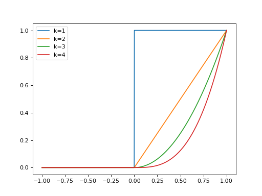
Bases: object

Causal Green function of the iterated derivative \(D^k\).

Examples

import matplotlib.pyplot as plt
import numpy as np
from pycsou.math.green import CausalGreenIteratedDerivative

x=np.linspace(-1,1,1024)
for k in range(1,5):
   green=CausalGreenIteratedDerivative(k)
   plt.plot(x, green(x))
plt.legend(['k=1', 'k=2', 'k=3', 'k=4'])

(Source code, png, hires.png, pdf)

Notes

The Green function \(\rho_k\) of the iterated derivative operator \(D^k\) on \(\mathbb{R}\) is defined as \(D^k\rho_k=\delta\). It is given by: \(\rho_k(t)\propto t^{k-1}_+\).

See also

CausalGreenExponential

__init__(k: int)

Parameters

k (int) – Exponent \(k\) of the iterated derivative operator \(D^k\) for which the Green function is desired.

class CausalGreenExponential(k: int, alpha: float = 1)

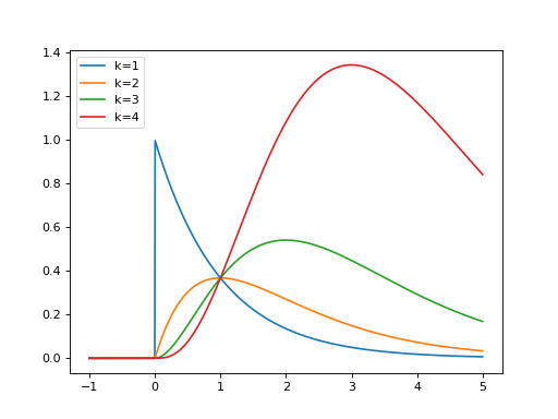
Bases: object

Causal Green function of \((D+\alpha\mbox{Id})^k\).

Examples

import matplotlib.pyplot as plt
import numpy as np
from pycsou.math.green import CausalGreenExponential

x=np.linspace(-1,5,1024)
for k in range(1,5):
   green=CausalGreenExponential(k)
   plt.plot(x, green(x))
plt.legend(['k=1', 'k=2', 'k=3', 'k=4'])

(Source code, png, hires.png, pdf)

Notes

The Green function \(\rho_k\) of the 1D pseudo-differential operator \((D+\alpha\mbox{Id})^k\) on \(\mathbb{R}\) is defined as \((D+\alpha\mbox{Id})^k\rho_k=\delta\). It is given by: \(\rho_k(t)\propto t_+^{k-1}e^{-\alpha t}\).

See also

CausalGreenIteratedDerivative

__init__(k: int, alpha: float = 1)

Parameters

• k (int) – Exponent \(k\) of the exponential pseudo-differential operator \((D+\alpha\mbox{Id})^k\) for which the Green function is desired.

• alpha (float) – Strictly positive parameter \(\alpha\) of the exponential pseudo-differential operator \((D+\alpha\mbox{Id})^k\) for which the Green function is desired.

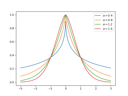
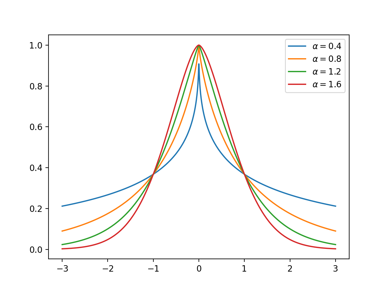
class SubGaussian(alpha: float, epsilon: float = 1.0)

Bases: object

Sub-Gaussian function.

Examples

import matplotlib.pyplot as plt
import numpy as np
from pycsou.math.green import SubGaussian

x=np.linspace(-3,3,1024)
lg=[]
for alpha in np.linspace(0,2,6)[1:-1]:
   subgaussian=SubGaussian(alpha)
   plt.plot(x, subgaussian(np.abs(x)))
   lg.append(f'$\\alpha={np.round(alpha,1)}$')
plt.legend(lg)

(Source code, png, hires.png, pdf)

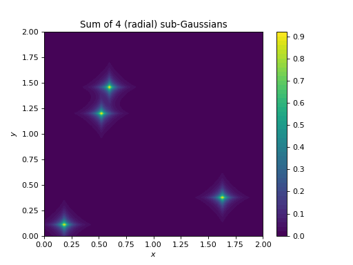
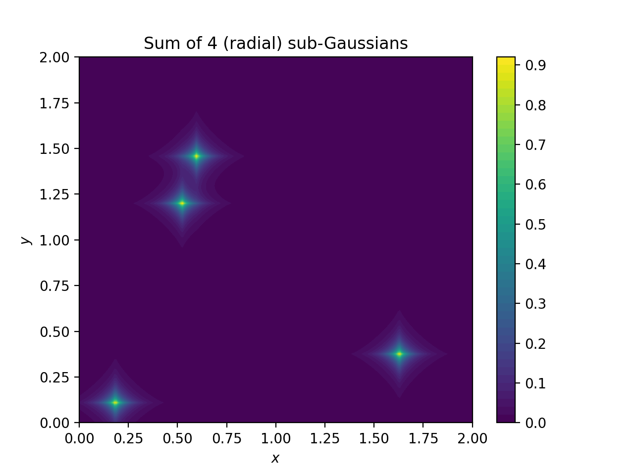
import numpy as np
import matplotlib.pyplot as plt
from pycsou.linop.sampling import MappedDistanceMatrix
from pycsou.math.green import SubGaussian

t = np.linspace(0, 2, 256)
rng = np.random.default_rng(seed=2)
x,y = np.meshgrid(t,t)
samples1 = np.stack((x.flatten(), y.flatten()), axis=-1)
samples2 = np.stack((2 * rng.random(size=4), 2 * rng.random(size=4)), axis=-1)
alpha = np.ones(samples2.shape[0])
ord=.8
epsilon = 1 / 12
func = SubGaussian(alpha=ord, epsilon=epsilon)
MDMOp = MappedDistanceMatrix(samples1=samples1, samples2=samples2, function=func, ord=ord, operator_type='dask')
plt.contourf(x,y,(MDMOp * alpha).reshape(t.size, t.size), 50)
plt.title('Sum of 4 (radial) sub-Gaussians')
plt.colorbar()
plt.xlabel('$x$')
plt.ylabel('$y$')

(Source code, png, hires.png, pdf)

Notes

The sub-Gaussian function is defined, for every \(\alpha\in (0,2)\) and \(\epsilon>0\), as:

\[f_\epsilon(r)=\exp\left(-\frac{r^\alpha}{\epsilon}\right), \qquad r\in \mathbb{R}_+.\]

It can be used to build sub-Gaussian radial kernels [SubGauss], which are known to be positive-definite and their inverse Fourier transforms (the so-called α-stable distributions) are heavy-tailed and infinitely smooth with algebraically decaying derivatives of any order.

__init__(alpha: float, epsilon: float = 1.0)

Parameters

• alpha (float) – Exponent \(\alpha\in (0,2)\) of the sub-Gaussian function.

• epsilon (float) – Spread \(\epsilon>0\) of the sub-Gaussian function.