Proximal Algorithms
Module: pycsou.opt.proxalgs
Proximal algorithms.
This module provides various proximal algorithms for convex optimisation.
|
Primal dual splitting algorithm. |
|
Accelerated proximal gradient descent. |
alias of |
|
|
Chambolle and Pock primal-dual splitting method. |
|
Douglas Rachford splitting algorithm. |
|
Forward-backward splitting algorithm. |
-
class
PrimalDualSplitting(dim: int, F: Optional[pycsou.core.map.DifferentiableMap] = None, G: Optional[pycsou.core.functional.ProximableFunctional] = None, H: Optional[pycsou.core.functional.ProximableFunctional] = None, K: Optional[pycsou.core.linop.LinearOperator] = None, tau: Optional[float] = None, sigma: Optional[float] = None, rho: Optional[float] = None, beta: Optional[float] = None, x0: Optional[numpy.ndarray] = None, z0: Optional[numpy.ndarray] = None, max_iter: int = 500, min_iter: int = 10, accuracy_threshold: float = 0.001, verbose: Optional[int] = 1)[source]¶ Bases:
pycsou.core.solver.GenericIterativeAlgorithmPrimal dual splitting algorithm.
This class is also accessible via the alias
PDS().Notes
The Primal Dual Splitting (PDS) method is described in [PDS] (this particular implementation is based on the pseudo-code Algorithm 7.1 provided in [FuncSphere] Chapter 7, Section1). It can be used to solve problems of the form:
\[{\min_{\mathbf{x}\in\mathbb{R}^N} \;\mathcal{F}(\mathbf{x})\;\;+\;\;\mathcal{G}(\mathbf{x})\;\;+\;\;\mathcal{H}(\mathbf{K} \mathbf{x}).}\]where:
\(\mathcal{F}:\mathbb{R}^N\rightarrow \mathbb{R}\) is convex and differentiable, with \(\beta\)-Lipschitz continuous gradient, for some \(\beta\in[0,+\infty[\).
\(\mathcal{G}:\mathbb{R}^N\rightarrow \mathbb{R}\cup\{+\infty\}\) and \(\mathcal{H}:\mathbb{R}^M\rightarrow \mathbb{R}\cup\{+\infty\}\) are two proper, lower semicontinuous and convex functions with simple proximal operators.
\(\mathbf{K}:\mathbb{R}^N\rightarrow \mathbb{R}^M\) is a linear operator, with operator norm:
\[\Vert{\mathbf{K}}\Vert_2=\sup_{\mathbf{x}\in\mathbb{R}^N,\Vert\mathbf{x}\Vert_2=1} \Vert\mathbf{K}\mathbf{x}\Vert_2.\]The problem is feasible –i.e. there exists at least one solution.
Remark 1:
The algorithm is still valid if one or more of the terms \(\mathcal{F}\), \(\mathcal{G}\) or \(\mathcal{H}\) is zero.
Remark 2:
Assume that the following holds:
\(\beta>0\) and:
\(\frac{1}{\tau}-\sigma\Vert\mathbf{K}\Vert_{2}^2\geq \frac{\beta}{2}\),
\(\rho \in ]0,\delta[\), where \(\delta:=2-\frac{\beta}{2}\left(\frac{1}{\tau}-\sigma\Vert\mathbf{K}\Vert_{2}^2\right)^{-1}\in[1,2[.\)
or \(\beta=0\) and:
\(\tau\sigma\Vert\mathbf{K}\Vert_{2}^2\leq 1\)
\(\rho \in [\epsilon,2-\epsilon]\), for some \(\epsilon>0.\)
Then, there exists a pair \((\mathbf{x}^\star,\mathbf{z}^\star)\in\mathbb{R}^N\times \mathbb{R}^M\)} solution s.t. the primal and dual sequences of estimates \((\mathbf{x}_n)_{n\in\mathbb{N}}\) and \((\mathbf{z}_n)_{n\in\mathbb{N}}\) converge towards \(\mathbf{x}^\star\) and \(\mathbf{z}^\star\) respectively, i.e.
\[\lim_{n\rightarrow +\infty}\Vert\mathbf{x}^\star-\mathbf{x}_n\Vert_2=0, \quad \text{and} \quad \lim_{n\rightarrow +\infty}\Vert\mathbf{z}^\star-\mathbf{z}_n\Vert_2=0.\]Default values of the hyperparameters provided here always ensure convergence of the algorithm.
Examples
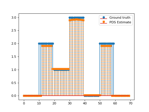
Consider the following optimisation problem:
\[\min_{\mathbf{x}\in\mathbb{R}_+^N}\frac{1}{2}\left\|\mathbf{y}-\mathbf{G}\mathbf{x}\right\|_2^2\quad+\quad\lambda_1 \|\mathbf{D}\mathbf{x}\|_1\quad+\quad\lambda_2 \|\mathbf{x}\|_1,\]with \(\mathbf{D}\in\mathbb{R}^{N\times N}\) the discrete derivative operator and \(\mathbf{G}\in\mathbb{R}^{L\times N}, \, \mathbf{y}\in\mathbb{R}^L, \lambda_1,\lambda_2>0.\) This problem can be solved via PDS with \(\mathcal{F}(\mathbf{x})= \frac{1}{2}\left\|\mathbf{y}-\mathbf{G}\mathbf{x}\right\|_2^2\), \(\mathcal{G}(\mathbf{x})=\lambda_2\|\mathbf{x}\|_1,\) \(\mathcal{H}(\mathbf{x})=\lambda \|\mathbf{x}\|_1\) and \(\mathbf{K}=\mathbf{D}\).
import numpy as np
import matplotlib.pyplot as plt
from pycsou.linop.diff import FirstDerivative
from pycsou.func.loss import SquaredL2Loss
from pycsou.func.penalty import L1Norm, NonNegativeOrthant
from pycsou.linop.sampling import DownSampling
from pycsou.opt.proxalgs import PrimalDualSplitting

x = np.repeat([0, 2, 1, 3, 0, 2, 0], 10)
D = FirstDerivative(size=x.size, kind='forward')
D.compute_lipschitz_cst(tol=1e-3)
rng = np.random.default_rng(0)
G = DownSampling(size=x.size, downsampling_factor=3)
G.compute_lipschitz_cst()
y = G(x)
l22_loss = (1 / 2) * SquaredL2Loss(dim=G.shape[0], data=y)
F = l22_loss * G
lambda_ = 0.1
H = lambda_ * L1Norm(dim=D.shape[0])
G = 0.01 * L1Norm(dim=G.shape[1])
pds = PrimalDualSplitting(dim=G.shape[1], F=F, G=G, H=H, K=D, verbose=None)
estimate, converged, diagnostics = pds.iterate()
plt.figure()
plt.stem(x, linefmt='C0-', markerfmt='C0o')
plt.stem(estimate['primal_variable'], linefmt='C1--', markerfmt='C1s')
plt.legend(['Ground truth', 'PDS Estimate'])
plt.show()
(Source code, png, hires.png, pdf)

See also
PDS,ChambollePockSplitting,DouglasRachford-
__init__(dim: int, F: Optional[pycsou.core.map.DifferentiableMap] = None, G: Optional[pycsou.core.functional.ProximableFunctional] = None, H: Optional[pycsou.core.functional.ProximableFunctional] = None, K: Optional[pycsou.core.linop.LinearOperator] = None, tau: Optional[float] = None, sigma: Optional[float] = None, rho: Optional[float] = None, beta: Optional[float] = None, x0: Optional[numpy.ndarray] = None, z0: Optional[numpy.ndarray] = None, max_iter: int = 500, min_iter: int = 10, accuracy_threshold: float = 0.001, verbose: Optional[int] = 1)[source]¶ - Parameters
dim (int) – Dimension of the objective functional’s domain.
F (Optional[DifferentiableMap]) – Differentiable map \(\mathcal{F}\).
G (Optional[ProximableFunctional]) – Proximable functional \(\mathcal{G}\).
H (Optional[ProximableFunctional]) – Proximable functional \(\mathcal{H}\).
K (Optional[LinearOperator]) – Linear operator \(\mathbf{K}\).
tau (Optional[float]) – Primal step size.
sigma (Optional[float]) – Dual step size.
rho (Optional[float]) – Momentum parameter.
beta (Optional[float]) – Lipschitz constant \(\beta\) of the derivative of \(\mathcal{F}\).
x0 (Optional[np.ndarray]) – Initial guess for the primal variable.
z0 (Optional[np.ndarray]) – Initial guess for the dual variable.
max_iter (int) – Maximal number of iterations.
min_iter (int) – Minimal number of iterations.
accuracy_threshold (float) – Accuracy threshold for stopping criterion.
verbose (int) – Print diagnostics every
verboseiterations. IfNonedoes not print anything.
-
set_step_sizes() → Tuple[float, float][source]¶ Set the primal/dual step sizes.
Notes
In practice, the convergence speed of the algorithm is improved by choosing \(\sigma\) and \(\tau\) as large as possible and relatively well-balanced –so that both the primal and dual variables converge at the same pace. In practice, it is hence recommended to choose perfectly balanced parameters \(\sigma=\tau\) saturating the convergence inequalities.
For \(\beta>0\) this yields:
\[\frac{1}{\tau}-\tau\Vert\mathbf{K}\Vert_{2}^2= \frac{\beta}{2} \quad\Longleftrightarrow\quad -2\tau^2\Vert\mathbf{K}\Vert_{2}^2-\beta\tau+2=0,\]which admits one positive root
\[\tau=\sigma=\frac{1}{\Vert\mathbf{K}\Vert_{2}^2}\left(-\frac{\beta}{4}+\sqrt{\frac{\beta^2}{16}+\Vert\mathbf{K}\Vert_{2}^2}\right).\]For \(\beta=0\), this yields
\[\tau=\sigma=\Vert\mathbf{K\Vert_{2}^{-1}.}\]
-
initialize_primal_variable() → numpy.ndarray[source]¶ Initialize the primal variable to zero.
- Returns
Zero-initialized primal variable.
- Return type
np.ndarray
-
PDS
-
class
AcceleratedProximalGradientDescent(dim: int, F: Optional[pycsou.core.map.DifferentiableMap] = None, G: Optional[pycsou.core.functional.ProximableFunctional] = None, tau: Optional[float] = None, acceleration: Optional[str] = 'CD', beta: Optional[float] = None, x0: Optional[numpy.ndarray] = None, max_iter: int = 500, min_iter: int = 10, accuracy_threshold: float = 0.001, verbose: Optional[int] = 1, d: float = 75.0)[source]¶ Bases:
pycsou.core.solver.GenericIterativeAlgorithmAccelerated proximal gradient descent.
This class is also accessible via the alias
APGD().Notes
The Accelerated Proximal Gradient Descent (APGD) method can be used to solve problems of the form:
\[{\min_{\mathbf{x}\in\mathbb{R}^N} \;\mathcal{F}(\mathbf{x})\;\;+\;\;\mathcal{G}(\mathbf{x}).}\]where:
\(\mathcal{F}:\mathbb{R}^N\rightarrow \mathbb{R}\) is convex and differentiable, with \(\beta\)-Lipschitz continuous gradient, for some \(\beta\in[0,+\infty[\).
\(\mathcal{G}:\mathbb{R}^N\rightarrow \mathbb{R}\cup\{+\infty\}\) is a proper, lower semicontinuous and convex function with a simple proximal operator.
The problem is feasible –i.e. there exists at least one solution.
Remark 1: the algorithm is still valid if one or more of the terms \(\mathcal{F}\) or \(\mathcal{G}\) is zero.
Remark 2: The convergence is guaranteed for step sizes \(\tau\leq 1/\beta\). Without acceleration, APGD can be seen as a PDS method with \(\rho=1\). The various acceleration schemes are described in [APGD]. For \(0<\tau\leq 1/\beta\) and Chambolle and Dossal’s acceleration scheme (
acceleration='CD'), APGD achieves the following (optimal) convergence rates:\[\lim\limits_{n\rightarrow \infty} n^2\left\vert \mathcal{J}(\mathbf{x}^\star)- \mathcal{J}(\mathbf{x}_n)\right\vert=0\qquad \&\qquad \lim\limits_{n\rightarrow \infty} n^2\Vert \mathbf{x}_n-\mathbf{x}_{n-1}\Vert^2_\mathcal{X}=0,\]for some minimiser \({\mathbf{x}^\star}\in\arg\min_{\mathbf{x}\in\mathbb{R}^N} \;\left\{\mathcal{J}(\mathbf{x}):=\mathcal{F}(\mathbf{x})+\mathcal{G}(\mathbf{x})\right\}\). In other words, both the objective functional and the APGD iterates \(\{\mathbf{x}_n\}_{n\in\mathbb{N}}\) converge at a rate \(o(1/n^2)\). In comparison Beck and Teboule’s acceleration scheme (
acceleration='BT') only achieves a convergence rate of \(O(1/n^2)\). Significant practical speedup can moreover be achieved for values of \(d\) in the range \([50,100]\) [APGD].Examples
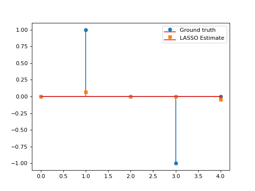
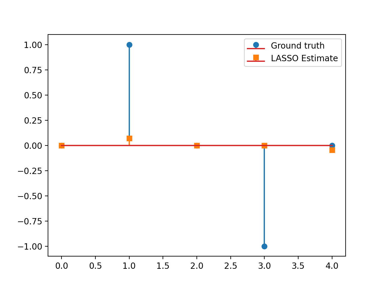
Consider the LASSO problem:
\[\min_{\mathbf{x}\in\mathbb{R}^N}\frac{1}{2}\left\|\mathbf{y}-\mathbf{G}\mathbf{x}\right\|_2^2\quad+\quad\lambda \|\mathbf{x}\|_1,\]with \(\mathbf{G}\in\mathbb{R}^{L\times N}, \, \mathbf{y}\in\mathbb{R}^L, \lambda>0.\) This problem can be solved via APGD with \(\mathcal{F}(\mathbf{x})= \frac{1}{2}\left\|\mathbf{y}-\mathbf{G}\mathbf{x}\right\|_2^2\) and \(\mathcal{G}(\mathbf{x})=\lambda \|\mathbf{x}\|_1\). We have:
\[\mathbf{\nabla}\mathcal{F}(\mathbf{x})=\mathbf{G}^T(\mathbf{G}\mathbf{x}-\mathbf{y}), \qquad \text{prox}_{\lambda\|\cdot\|_1}(\mathbf{x})=\text{soft}_\lambda(\mathbf{x}).\]This yields the so-called Fast Iterative Soft Thresholding Algorithm (FISTA), whose convergence is guaranteed for \(d>2\) and \(0<\tau\leq \beta^{-1}=\|\mathbf{G}\|_2^{-2}\).
import numpy as np
import matplotlib.pyplot as plt
from pycsou.func.loss import SquaredL2Loss
from pycsou.func.penalty import L1Norm
from pycsou.linop.base import DenseLinearOperator
from pycsou.opt.proxalgs import APGD

rng = np.random.default_rng(0)
G = DenseLinearOperator(rng.standard_normal(15).reshape(3,5))
G.compute_lipschitz_cst()
x = np.zeros(G.shape[1])
x[1] = 1
x[-2] = -1
y = G(x)
l22_loss = (1/2) * SquaredL2Loss(dim=G.shape[0], data=y)
F = l22_loss * G
lambda_ = 0.9 * np.max(np.abs(F.gradient(0 * x)))
G = lambda_ * L1Norm(dim=G.shape[1])
apgd = APGD(dim=G.shape[1], F=F, G=G, acceleration='CD', verbose=None)
estimate, converged, diagnostics = apgd.iterate()
plt.figure()
plt.stem(x, linefmt='C0-', markerfmt='C0o')
plt.stem(estimate['iterand'], linefmt='C1--', markerfmt='C1s')
plt.legend(['Ground truth', 'LASSO Estimate'])
plt.show()
(Source code, png, hires.png, pdf)

See also
-
__init__(dim: int, F: Optional[pycsou.core.map.DifferentiableMap] = None, G: Optional[pycsou.core.functional.ProximableFunctional] = None, tau: Optional[float] = None, acceleration: Optional[str] = 'CD', beta: Optional[float] = None, x0: Optional[numpy.ndarray] = None, max_iter: int = 500, min_iter: int = 10, accuracy_threshold: float = 0.001, verbose: Optional[int] = 1, d: float = 75.0)[source]¶ - Parameters
dim (int) – Dimension of the objective functional’s domain.
F (Optional[DifferentiableMap]) – Differentiable map \(\mathcal{F}\).
G (Optional[ProximableFunctional]) – Proximable functional \(\mathcal{G}\).
tau (Optional[float]) – Primal step size.
acceleration (Optional[str] [None, 'BT', 'CD']) – Which acceleration scheme should be used (None for no acceleration).
beta (Optional[float]) – Lipschitz constant \(\beta\) of the derivative of \(\mathcal{F}\).
x0 (Optional[np.ndarray]) – Initial guess for the primal variable.
max_iter (int) – Maximal number of iterations.
min_iter (int) – Minimal number of iterations.
accuracy_threshold (float) – Accuracy threshold for stopping criterion.
verbose (int) – Print diagnostics every
verboseiterations. IfNonedoes not print anything.d (float) – Parameter \(d\) for Chambolle and Dossal’s acceleration scheme (
acceleration='CD').
-
APGD¶ alias of
pycsou.opt.proxalgs.AcceleratedProximalGradientDescent
-
class
ChambollePockSplitting(dim: int, G: Optional[pycsou.core.functional.ProximableFunctional] = None, H: Optional[pycsou.core.functional.ProximableFunctional] = None, K: Optional[pycsou.core.linop.LinearOperator] = None, tau: Optional[float] = None, sigma: Optional[float] = None, rho: Optional[float] = 1, x0: Optional[numpy.ndarray] = None, z0: Optional[numpy.ndarray] = None, max_iter: int = 500, min_iter: int = 10, accuracy_threshold: float = 0.001, verbose: Optional[int] = 1)[source]¶ Bases:
pycsou.opt.proxalgs.PrimalDualSplittingChambolle and Pock primal-dual splitting method.
This class is also accessible via the alias
CPS().Notes
The Chambolle and Pock primal-dual splitting (CPS) method can be used to solve problems of the form:
\[{\min_{\mathbf{x}\in\mathbb{R}^N} \mathcal{G}(\mathbf{x})\;\;+\;\;\mathcal{H}(\mathbf{K} \mathbf{x}).}\]where:
\(\mathcal{G}:\mathbb{R}^N\rightarrow \mathbb{R}\cup\{+\infty\}\) and \(\mathcal{H}:\mathbb{R}^M\rightarrow \mathbb{R}\cup\{+\infty\}\) are two proper, lower semicontinuous and convex functions with simple proximal operators.
\(\mathbf{K}:\mathbb{R}^N\rightarrow \mathbb{R}^M\) is a linear operator, with operator norm:
\[\Vert{\mathbf{K}}\Vert_2=\sup_{\mathbf{x}\in\mathbb{R}^N,\Vert\mathbf{x}\Vert_2=1} \Vert\mathbf{K}\mathbf{x}\Vert_2.\]The problem is feasible –i.e. there exists at least one solution.
Remark 1:
The algorithm is still valid if one of the terms \(\mathcal{G}\) or \(\mathcal{H}\) is zero.
Remark 2:
Assume that the following holds:
\(\tau\sigma\Vert\mathbf{K}\Vert_{2}^2\leq 1\)
\(\rho \in [\epsilon,2-\epsilon]\), for some \(\epsilon>0.\)
Then, there exists a pair \((\mathbf{x}^\star,\mathbf{z}^\star)\in\mathbb{R}^N\times \mathbb{R}^M\)} solution s.t. the primal and dual sequences of estimates \((\mathbf{x}_n)_{n\in\mathbb{N}}\) and \((\mathbf{z}_n)_{n\in\mathbb{N}}\) converge towards \(\mathbf{x}^\star\) and \(\mathbf{z}^\star\) respectively, i.e.
\[\lim_{n\rightarrow +\infty}\Vert\mathbf{x}^\star-\mathbf{x}_n\Vert_2=0, \quad \text{and} \quad \lim_{n\rightarrow +\infty}\Vert\mathbf{z}^\star-\mathbf{z}_n\Vert_2=0.\]Default values of the hyperparameters provided here always ensure convergence of the algorithm.
See also
-
__init__(dim: int, G: Optional[pycsou.core.functional.ProximableFunctional] = None, H: Optional[pycsou.core.functional.ProximableFunctional] = None, K: Optional[pycsou.core.linop.LinearOperator] = None, tau: Optional[float] = None, sigma: Optional[float] = None, rho: Optional[float] = 1, x0: Optional[numpy.ndarray] = None, z0: Optional[numpy.ndarray] = None, max_iter: int = 500, min_iter: int = 10, accuracy_threshold: float = 0.001, verbose: Optional[int] = 1)[source]¶ - Parameters
dim (int) – Dimension of the objective functional’s domain.
G (Optional[ProximableFunctional]) – Proximable functional \(\mathcal{G}\).
H (Optional[ProximableFunctional]) – Proximable functional \(\mathcal{H}\).
K (Optional[LinearOperator]) – Linear operator \(\mathbf{K}\).
tau (Optional[float]) – Primal step size.
sigma (Optional[float]) – Dual step size.
rho (Optional[float]) – Momentum parameter.
x0 (Optional[np.ndarray]) – Initial guess for the primal variable.
z0 (Optional[np.ndarray]) – Initial guess for the dual variable.
max_iter (int) – Maximal number of iterations.
min_iter (int) – Minimal number of iterations.
accuracy_threshold (float) – Accuracy threshold for stopping criterion.
verbose (int) – Print diagnostics every
verboseiterations. IfNonedoes not print anything.
-
CPS
-
class
DouglasRachfordSplitting(dim: int, G: Optional[pycsou.core.functional.ProximableFunctional] = None, H: Optional[pycsou.core.functional.ProximableFunctional] = None, tau: float = 1.0, x0: Optional[numpy.ndarray] = None, z0: Optional[numpy.ndarray] = None, max_iter: int = 500, min_iter: int = 10, accuracy_threshold: float = 0.001, verbose: Optional[int] = 1)[source]¶ Bases:
pycsou.opt.proxalgs.PrimalDualSplittingDouglas Rachford splitting algorithm.
This class is also accessible via the alias
DRS().Notes
The Douglas Rachford Splitting (DRS) can be used to solve problems of the form:
\[{\min_{\mathbf{x}\in\mathbb{R}^N} \mathcal{G}(\mathbf{x})\;\;+\;\;\mathcal{H}(\mathbf{x}).}\]where:
\(\mathcal{G}:\mathbb{R}^N\rightarrow \mathbb{R}\cup\{+\infty\}\) and \(\mathcal{H}:\mathbb{R}^M\rightarrow \mathbb{R}\cup\{+\infty\}\) are two proper, lower semicontinuous and convex functions with simple proximal operators.
The problem is feasible –i.e. there exists at least one solution.
Remark 1:
The algorithm is still valid if one of the terms \(\mathcal{G}\) or \(\mathcal{H}\) is zero.
Default values of the hyperparameters provided here always ensure convergence of the algorithm.
See also
-
__init__(dim: int, G: Optional[pycsou.core.functional.ProximableFunctional] = None, H: Optional[pycsou.core.functional.ProximableFunctional] = None, tau: float = 1.0, x0: Optional[numpy.ndarray] = None, z0: Optional[numpy.ndarray] = None, max_iter: int = 500, min_iter: int = 10, accuracy_threshold: float = 0.001, verbose: Optional[int] = 1)[source]¶ - Parameters
dim (int) – Dimension of the objective functional’s domain.
G (Optional[ProximableFunctional]) – Proximable functional \(\mathcal{G}\).
H (Optional[ProximableFunctional]) – Proximable functional \(\mathcal{H}\).
tau (Optional[float]) – Primal step size.
x0 (Optional[np.ndarray]) – Initial guess for the primal variable.
z0 (Optional[np.ndarray]) – Initial guess for the dual variable.
max_iter (int) – Maximal number of iterations.
min_iter (int) – Minimal number of iterations.
accuracy_threshold (float) – Accuracy threshold for stopping criterion.
verbose (int) – Print diagnostics every
verboseiterations. IfNonedoes not print anything.
-
DRS
-
class
ForwardBackwardSplitting(dim: int, F: Optional[pycsou.core.functional.DifferentiableFunctional] = None, G: Optional[pycsou.core.functional.ProximableFunctional] = None, tau: Optional[float] = None, rho: Optional[float] = 1, x0: Optional[numpy.ndarray] = None, max_iter: int = 500, min_iter: int = 10, accuracy_threshold: float = 0.001, verbose: Optional[int] = 1)[source]¶ Bases:
pycsou.opt.proxalgs.PrimalDualSplittingForward-backward splitting algorithm.
This class is also accessible via the alias
FBS().Notes
The Forward-backward splitting (FBS) method can be used to solve problems of the form:
\[{\min_{\mathbf{x}\in\mathbb{R}^N} \;\mathcal{F}(\mathbf{x})\;\;+\;\;\mathcal{G}(\mathbf{x}).}\]where:
\(\mathcal{F}:\mathbb{R}^N\rightarrow \mathbb{R}\) is convex and differentiable, with \(\beta\)-Lipschitz continuous gradient, for some \(\beta\in[0,+\infty[\).
\(\mathcal{G}:\mathbb{R}^N\rightarrow \mathbb{R}\cup\{+\infty\}\) is proper, lower semicontinuous and convex function with simple proximal operator.
The problem is feasible –i.e. there exists at least one solution.
Remark 1:
The algorithm is still valid if one of the terms \(\mathcal{F}\) or \(\mathcal{G}\) is zero.
Remark 2:
Assume that the following holds:
\(\frac{1}{\tau}\geq \frac{\beta}{2}\),
\(\rho \in ]0,\delta[\), where \(\delta:=2-\frac{\beta}{2}\tau\in[1,2[.\)
Then, there exists a pair \((\mathbf{x}^\star,\mathbf{z}^\star)\in\mathbb{R}^N\times \mathbb{R}^M\)} solution s.t. the primal and dual sequences of estimates \((\mathbf{x}_n)_{n\in\mathbb{N}}\) and \((\mathbf{z}_n)_{n\in\mathbb{N}}\) converge towards \(\mathbf{x}^\star\) and \(\mathbf{z}^\star\) respectively, i.e.
\[\lim_{n\rightarrow +\infty}\Vert\mathbf{x}^\star-\mathbf{x}_n\Vert_2=0, \quad \text{and} \quad \lim_{n\rightarrow +\infty}\Vert\mathbf{z}^\star-\mathbf{z}_n\Vert_2=0.\]Default values of the hyperparameters provided here always ensure convergence of the algorithm.
See also
-
__init__(dim: int, F: Optional[pycsou.core.functional.DifferentiableFunctional] = None, G: Optional[pycsou.core.functional.ProximableFunctional] = None, tau: Optional[float] = None, rho: Optional[float] = 1, x0: Optional[numpy.ndarray] = None, max_iter: int = 500, min_iter: int = 10, accuracy_threshold: float = 0.001, verbose: Optional[int] = 1)[source]¶ - Parameters
dim (int) – Dimension of the objective functional’s domain.
F (Optional[DifferentiableMap]) – Differentiable map \(\mathcal{F}\).
G (Optional[ProximableFunctional]) – Proximable functional \(\mathcal{G}\).
tau (Optional[float]) – Primal step size.
rho (Optional[float]) – Momentum parameter.
beta (Optional[float]) – Lipschitz constant \(\beta\) of the derivative of \(\mathcal{F}\).
x0 (Optional[np.ndarray]) – Initial guess for the primal variable.
max_iter (int) – Maximal number of iterations.
min_iter (int) – Minimal number of iterations.
accuracy_threshold (float) – Accuracy threshold for stopping criterion.
verbose (int) – Print diagnostics every
verboseiterations. IfNonedoes not print anything.
-
FBS