Solving Inverse Problems with Pycsou

Pycsou is a Python 3 package for solving linear inverse problems with state-of-the-art proximal algorithms. The library provides abstract classes for the main building blocks of generic penalised convex optimisation problems:

• linear operators,

• loss functionals,

• penalty functionals,

• proximal algorithms.

Penalised convex optimisation problems can then be constructed by adding, subtracting, scaling, composing, exponentiating or stacking together the various linear operators and functionals shipped with Pycsou (or custom, user-defined ones).

Multidimensional Maps

Pycsou’s base classes for functionals and linear operators both inherit from the abstract class Map with signature:

class Map(shape: Tuple[int, int], is_linear: bool = False,
          is_differentiable: bool = False):

This is the base class for multidimensional maps (potentially nonlinear) \(\mathbf{h}:\mathbb{R}^M\to\mathbb{R}^N\).

Any instance/subclass of this class must at least implement the abstract method __call__ for pointwise evaluation.

Operations on Map Instances

The class Map supports the following arithmetic operators +, -, *, @, ** and /, implemented with the class methods __add__/__radd__, __sub__/__neg__, __mul__/__rmul__, __matmul__, __pow__,__truediv__. Such arithmetic operators can be used to add, substract, scale, compose, exponentiate or evaluate Map instances. The __call__ methods of Map objects constructed this way are automatically computed:

>>> f3 = f1 / 3 + np.pi * f2
>>> np.allclose(f3(x), f1(x) / 3 + np.pi * f2(x))
True
>>> h3 = h1 * 3 - (h2 ** 2) / 6
>>> np.allclose(h3(x), h1(x) * 3 - (h2(h2(x))) / 6)
True

Note that multiplying a map with an array is the same as evaluating the map at the array:

>>> np.allclose(h * x, h(x))
True

The multiplication operator @ can also be used in place of *, in compliance with Numpy’s interface:

>>> np.allclose(h * x, h @ x), np.allclose((h1 * h2)(x), (h1 @ h2)(x))
True, True

Finally, maps can be shifted via the method shifter:

>>> h=g.shifter(shift=2 * x)
>>> np.allclose(h(x), g(x + 2 * x))
True

Differentiable Maps

An important subclass of Map is DifferentiableMap which is the base class for differentiable maps. It has the following signature:

class DifferentiableMap(shape: Tuple[int, int],is_linear: bool = False,
                        lipschitz_cst: float = inf,
                        diff_lipschitz_cst: float = inf):

Any instance/subclass of this class must implement the abstract methods __call__ and jacobianT which returns the transpose of the Jacobian matrix

\[(\mathbf{J}_{\mathbf{h}}(\mathbf{x}))_{ij}:=\frac{\partial h_i}{\partial x_j}(\mathbf{x})\]

of the multidimensional \(\mathbf{h}=[h_1, \ldots, h_N]: \mathbb{R}^M\to\mathbb{R}^N\) at a given point \(\mathbf{x}\in\mathbb{R}^M\).

Operations on DifferentiableMap Instances

Standard arithmetic operators can also be used on DifferentiableMap instances so as to add, substract, scale, compose, exponentiate or evaluate them. The attributes lipschitz_cst, diff_lipschitz_cst and the method jacobianT are automatically updated using standard differentiation rules.

>>> map_ = f * g
>>> np.allclose(map_.lipschitz_cst, f.lipschitz_cst * g.lipschitz_cst)
True
>>> np.allclose(map_.jacobianT(x), g.jacobianT(x) * f.jacobianT(g(x)))
True

Functionals

Functionals are (real) single-valued maps \(h:\mathbb{R}^N\to \mathbb{R}\). They can be implemented via a subclass of Map called Functional:

class Functional(dim: int,
                 data: Optional[numpy.ndarray] = None,
                 is_differentiable: bool = False,
                 is_linear: bool = False)

For differentiable functionals, the subclass DifferentiableFunctional can be used. The latter admits a method gradient which is an alias for the abstract method jacobianT.

Note

Reminder: for a functional \(h\), \(\mathbf{J}^T_h(\mathbf{x})=\nabla h (\mathbf{x})\).

Proximable Functionals

We say that a functional \(f:\mathbb{R}^N\to \mathbb{R}\) is proximable is its proximity operator

\[\mathbf{\text{prox}}_{\tau f}(\mathbf{z}):=\arg\min_{\mathbf{x}\in\mathbb{R}^N} f(x)+\frac{1}{2\tau} \|\mathbf{x}-\mathbf{z}\|_2^2, \quad \forall \mathbf{z}\in\mathbb{R}^N,\]

admits a simple closed-form expression or can be evaluated efficiently and with high accuracy.

They are represented by the subclass ProximableFunctional. The latter has signature:

class ProximableFunctional(dim: int,
                           data: Optional[numpy.ndarray] = None,
                           is_differentiable: bool = False,
                           is_linear: bool = False)

Every subclass/instance of ProximableFunctional must at least implement the abstract methods __call__ and prox.

Note

See Cost Functionals for a list of common functionals already implemented in Pycsou.

Operations on Proximable Functionals

For the following basic operations, the proximal operator can be automatically updated:

• Postcomposition: \(g(\mathbf{x})=\alpha f(\mathbf{x})\),

• Precomposition: \(g(\mathbf{x})= f(\alpha\mathbf{x}+b)\) or \(g(\mathbf{x})= f(U\mathbf{x})\) with \(U\) a unitary operator,

• Affine Sum: \(g(\mathbf{x})= f(\mathbf{x})+\mathbf{a}^T\mathbf{x}.\)

>>> from pycsou.func.penalty import L1Norm
>>> func = L1Norm(dim=10)
>>> x = np.arange(10); tau=0.1
>>> np.allclose((2 * func).prox(x, tau), func.prox(x, 2 * tau))
True
>>> np.allclose((func * 2).prox(x, tau), func.prox(x * 2, 4 * tau)/2)
True
>>> np.allclose(func.shifter(x/2).prox(x, tau), func.prox(x+x/2, tau)-x/2)
True

Horizontal Stacking of Proximable Functionals

The class ProxFuncHStack allows to stack many functionals \(\{f_i:\mathbb{R}^{N_i}\to \mathbb{R}, i=1,\ldots, k\}\) horizontally:

\[\begin{split}h:\begin{cases}\mathbb{R}^{N_1}\times \cdots \times\mathbb{R}^{N_k}\to \mathbb{R}\\ (\mathbf{x}_1,\ldots, \mathbf{x}_k)\mapsto \sum_{i=1}^k f_i(\mathbf{x}_i). \end{cases}\end{split}\]

The proximity operator of the stacked functional \(h\) is moreover computed automatically (and soon in parallel) via the formula:

\[\mathbf{\text{prox}}_{\tau h}(\mathbf{x}_1,\ldots, \mathbf{x}_k)=\left(\mathbf{\text{prox}}_{\tau f_1}(\mathbf{x}_1),\ldots, \mathbf{\text{prox}}_{\tau f_k}(\mathbf{x}_k)\right).\]

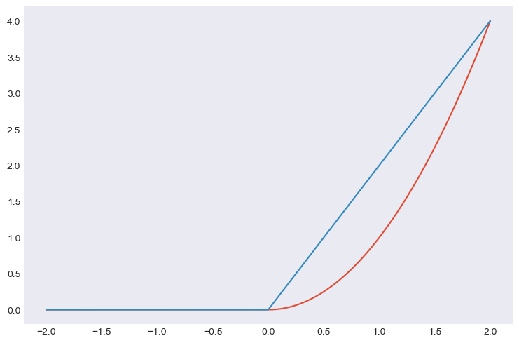
Example: Implementing New Differentiable Functionals

from pycsou.core import DifferentiableFunctional

class OneSidedSquaredL2Norm(DifferentiableFunctional):
    def __init__(self, dim: int):
        super(OneSidedSquaredL2Norm, self).__init__(dim=dim, diff_lipschitz_cst=2)

    def __call__(self, x: np.ndarray) -> np.ndarray: #Implement abstract method __call__
        return np.sum(x**2 * (x >= 0))

    def jacobianT(self, x: np.ndarray) -> np.ndarray: #Implement abstract method jacobianT
        return 2 * x * (x >= 0)

x=np.linspace(-2,2,1000)
func=OneSidedSquaredL2Norm(dim=1)
y = [func(t) for t in x]; dy = [func.gradient(t) for t in x]
plt.plot(x,y); plt.plot(x,dy)

Linear Operators

The base class for linear operators \(\mathbf{L}:\mathbb{R}^N\to \mathbb{R}^M\) is LinearOperator, a subclass of DifferentiableMap with signature:

class LinearOperator(shape: Tuple[int, int], dtype: Optional[type] = None,
                    is_explicit: bool = False, is_dense: bool = False,
                    is_sparse: bool = False, is_dask: bool = False,
                    is_symmetric: bool = False,
                    lipschitz_cst: float = inf)

Any instance/subclass of this class must at least implement the abstract methods __call__ for forward evaluation \(\mathbf{L}\mathbf{x}\) and adjoint for backward evaluation \(\mathbf{L}^\ast\mathbf{y}\) where \(\mathbf{L}^\ast:\mathbb{R}^M\to \mathbb{R}^N\) is the adjoint of \(\mathbf{L}\) defined as:

\[\langle \mathbf{x}, \mathbf{L}^\ast\mathbf{y}\rangle_{\mathbb{R}^N}:=\langle \mathbf{L}\mathbf{x}, \mathbf{y}\rangle_{\mathbb{R}^M}, \qquad\forall (\mathbf{x},\mathbf{y})\in \mathbb{R}^N\times \mathbb{R}^M.\]

Matrix-Free Operators

Pycsou’s linear operators are inherently matrix-free: the operator \(\mathbf{L}\) needs not be stored as an array since the methods __call__ (alias matvec) and adjoint can be used to perform matrix-vector products \(\mathbf{L}\mathbf{x}\) and \(\mathbf{L}^\ast\mathbf{y}\) respectively. This is particularly useful when the dimensions \(N\) and \(M\) are very large (e.g. in image processing) and \(\mathbf{L}\) cannot be stored in memory as a Numpy array.

The class LinearOperator can be thought as an interface-compatible overload of the standard matrix-free classes pylops.LinearOperator and scipy.sparse.linalg.LinearOperator from PyLops and Scipy respectively.

Pycsou’s LinearOperator introduces notably the method jacobianT, useful for automatic differentiation when composing linear operators with differentiable functionals:

\[\mathbf{J}^T_{\mathbf{L}}(\mathbf{x}):=\mathbf{L}^T, \;\forall\mathbf{x}\in\mathbb{R}^N.\]

It also introduces convenience linear algebra methods such as eigenvals, svds, pinv, cond, etc.

Note

See Linear Operators for a list of matrix-free linear operators already implemented in Pycsou.

Explicit Operators

Sometimes it can be cumbersome to specify an operator in matrix-free form. In which case, Pycsou’s class ExplicitLinearOperator can be used to construct linear operators from array-like representations:

class ExplicitLinearOperator(array: Union[numpy.ndarray,
                                          scipy.sparse.base.spmatrix,
                                          dask.array.core.Array],
                             is_symmetric: bool = False)

This class takes as input Numpy arrays, Scipy sparse matrices (in any sparse format) or Dask distributed arrays.

Finally, matrix-free operators can be converted into explicit operators via the methods todense or tosparse (useful for visualisation/debugging but often memory intensive).

Operations on Linear Operators

Just like DifferentiableMap, the class LinearOperator supports the whole set of arithmetic operations: +, -, *, @, ** and /. ’

The abstract methods __call__, jacobianT and adjoint of LinearOperator instances resulting from arithmetic operations are automatically updated.

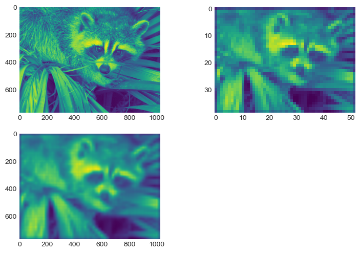
from pycsou.linop import Convolve2D, DownSampling

input_image = face(gray=True)
filter_size = 40
filter_support = np.linspace(-3, 3, filter_size)
gaussian_filter = np.exp(-(filter_support[:, None]
                           ** 2 + filter_support[None, :] ** 2) / 2 * (0.5))

FilterOp = Convolve2D(size=input_image.size,
                      filter=gaussian_filter, shape=input_image.shape)
DownSamplingOp = DownSampling(
    size=input_image.size, downsampling_factor=20, shape=input_image.shape)
BlurringOp = DownSamplingOp * FilterOp # Compose a filtering operator with a downsampling operator.

blurred_image = (BlurringOp * input_image.flatten()
                 ).reshape(DownSamplingOp.output_shape) # Method __call__ of composite operator is available.
backproj_image = BlurringOp.adjoint(
    blurred_image.flatten()).reshape(input_image.shape) # Method adjoint of composite operator is available.

plt.figure()
plt.subplot(2, 2, 1)
plt.imshow(input_image)
plt.subplot(2, 2, 2)
plt.imshow(blurred_image)
plt.subplot(2, 2, 3)
plt.imshow(backproj_image)

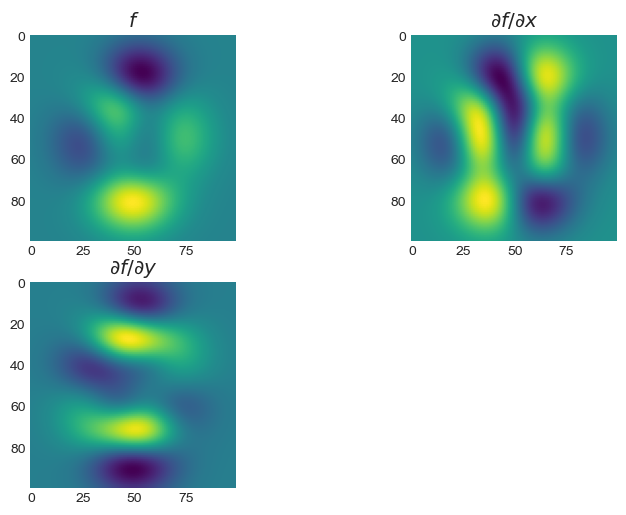
It is also possible to stack LinearOperator instances horizontally/vertically via the class LinOpStack:

from pycsou.linop import FirstDerivative, LinOpStack
from pycsou.util import peaks

x = np.linspace(-2.5, 2.5, 100)
X,Y = np.meshgrid(x,x)
Z = peaks(X, Y)

D1 = FirstDerivative(size=Z.size, shape=Z.shape, axis=1,
                         kind='centered')
D2 = FirstDerivative(size=Z.size, shape=Z.shape, axis=0,
                         kind='centered')
Gradient = LinOpStack(D1, D2, axis=0) # Form the gradient by stacking 1D derivative operators

DZ=Gradient(Z.flatten())

plt.figure(); plt.subplot(2,2,1)
plt.imshow(Z)
plt.title('$f$'); plt.subplot(2,2,2)
plt.imshow(DZ[:Z.size].reshape(Z.shape))
plt.title('$\\partial f/\\partial x$'); plt.subplot(2,2,3)
plt.imshow(DZ[Z.size:].reshape(Z.shape))
plt.title('$\\partial f/\\partial y$')

Example: Implementing New Linear Operators

from pycsou.core import LinearOperator

class RepCol(LinearOperator):
    def __init__(self, size: int, reps: int, dtype: type = np.float64):
        self.reps = reps
        super(RepCol, self).__init__(shape=(size*reps, size))

    def __call__(self, x: np.ndarray) -> np.ndarray:
        return np.tile(x[:,None], (1, self.reps)).flatten()

    def adjoint(self, y: np.ndarray) -> np.ndarray:
        return np.sum(y.reshape(self.shape[1], reps), axis=-1).flatten()

x =np.arange(4)
Op=RepCol(x.size, 5)
y=Op(x).reshape(x.size,5)
print(y)

[[0 0 0 0 0]
 [1 1 1 1 1]
 [2 2 2 2 2]
 [3 3 3 3 3]]

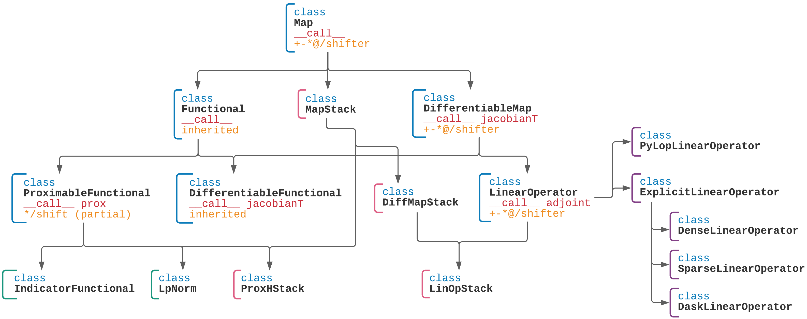
Pycsou Class Diagram

Algorithms

The base class for Pycsou’s iterative algorithms is GenericIterativeAlgorithm:

class GenericIterativeAlgorithm(objective_functional: pycsou.core.map.Map,
                                init_iterand: Any,
                                max_iter: int = 500,
                                min_iter: int = 10,
                                accuracy_threshold: float = 0.001,
                                verbose: Optional[int] = None)

Any instance/subclass of this class must at least implement the abstract methods update_iterand, print_diagnostics, update_diagnostics and stopping_metric.

Primal Dual Splitting Method (PDS)

Most algorithms shipped with Pycsou (FBS, APGD, ADMM, CPS, DRS, etc) are special cases of Condat’s primal-dual splitting method (PDS) implemented in the class PrimalDualSplitting (alias PDS):

class PrimalDualSplitting(dim: int,
                          F: Optional[DifferentiableMap] = None,
                          G: Optional[ProximableFunctional] = None,
                          H: Optional[ProximableFunctional] = None,
                          K: Optional[LinearOperator] = None,
                          tau: Optional[float] = None,
                          sigma: Optional[float] = None,
                          rho: Optional[float] = None,
                          beta: Optional[float] = None,
                          ...)

The user must simply put its problem in the form \({\min_{\mathbf{x}\in\mathbb{R}^N} \;\mathcal{F}(\mathbf{x})\;\;+\;\;\mathcal{G}(\mathbf{x})\;\;+\;\;\mathcal{H}(\mathbf{K} \mathbf{x})}\) and provide the relevant terms to the class constructor.

See also

See Proximal Algorithms for implementations of the above mentionned algorithms in Pycsou.

Hyperparameters Auto-tuning

For convergence of the algorithm, the step sizes/momentum parameter \(\tau\), \(\sigma\) and \(\rho\) must verify:

• If the Lipschitz constant \(\beta\) of \(\nabla \mathcal{F}\) is positive:

  • \(\frac{1}{\tau}-\sigma\Vert\mathbf{K}\Vert_{2}^2\geq \frac{\beta}{2}\),

  • \(\rho \in ]0,\delta[\), where \(\delta:=2-\frac{\beta}{2}\left(\frac{1}{\tau}-\sigma\Vert\mathbf{K}\Vert_{2}^2\right)^{-1}\in[1,2[.\)

• If the Lipschitz constant \(\beta\) of \(\nabla \mathcal{F}\) is null (e.g. \(\mathcal{F}=0\)):

  • \(\tau\sigma\Vert\mathbf{K}\Vert_{2}^2\leq 1\)

  • \(\rho \in [\epsilon,2-\epsilon]\), for some \(\epsilon>0.\)

When the user does not specify hyperparameters, we choose the step sizes as large as possible and perfectly balanced (improves practical convergence speed):

• \(\beta>0\):

  \[\tau=\sigma=\frac{1}{\Vert\mathbf{K}\Vert_{2}^2}\left(-\frac{\beta}{4}+\sqrt{\frac{\beta^2}{16}+\Vert\mathbf{K}\Vert_{2}^2}\right).\]

• \(\beta=0\):

  \[\tau=\sigma=\Vert\mathbf{K}\Vert_{2}^{-1}.\]

The momentum term \(\rho\) is chosen as \(\rho=0.9\) (\(\beta>0\)) or \(\rho=1\) (\(\beta=0\)).

Note

\(\Vert\mathbf{K}\Vert_{2}\) can be computed efficiently via the method LinearOperator.compute_lipschitz_cst which relies on Scipy’s sparse linear algebra routines eigs/eigsh/svds.

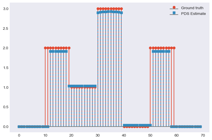
Example:

\[\min_{\mathbf{x}\in\mathbb{R}^N}\frac{1}{2}\left\|\mathbf{y}-\mathbf{G}\mathbf{x}\right\|_2^2\quad+\quad\lambda_1 \|\mathbf{D}\mathbf{x}\|_1\quad+\quad\lambda_2 \|\mathbf{x}\|_1,\]

with \(\mathbf{D}\in\mathbb{R}^{N\times N}\) and \(\mathbf{G}\in\mathbb{R}^{L\times N}, \, \mathbf{y}\in\mathbb{R}^L, \lambda_1,\lambda_2>0.\) This problem can be written in the form

\[{\min_{\mathbf{x}\in\mathbb{R}^N} \;\mathcal{F}(\mathbf{x})\;\;+\;\;\mathcal{G}(\mathbf{x})\;\;+\;\;\mathcal{H}(\mathbf{K} \mathbf{x})}\]

by choosing \(\mathcal{F}(\mathbf{x})= \frac{1}{2}\left\|\mathbf{y}-\mathbf{G}\mathbf{x}\right\|_2^2\), \(\mathcal{G}(\mathbf{x})=\lambda_2\|\mathbf{x}\|_1\), \(\mathcal{H}(\mathbf{x})=\lambda_1 \|\mathbf{x}\|_1\) and \(\mathbf{K}=\mathbf{D}\).

from pycsou.linop import FirstDerivative, DownSampling
from pycsou.func import SquaredL2Loss, L1Norm, NonNegativeOrthant
from pycsou.opt import PrimalDualSplitting

x = np.repeat([0, 2, 1, 3, 0, 2, 0], 10) # Ground truth
D = FirstDerivative(size=x.size, kind='forward') # Regularisation operator
D.compute_lipschitz_cst(tol=1e-3)
G = DownSampling(size=x.size, downsampling_factor=3) # Downsampling operator
G.compute_lipschitz_cst() # Compute Lipschitz constant for automatic parameter tuning
y = G(x) # Input data (downsampled x)

l22_loss = (1 / 2) * SquaredL2Loss(dim=G.shape[0], data=y) # Least-squares loss
F = l22_loss * G # Differentiable term F
H = 0.1 * L1Norm(dim=D.shape[0]) # Proximable term H
G = 0.01 * L1Norm(dim=G.shape[1]) # Proximable term F
pds = PrimalDualSplitting(dim=G.shape[1], F=F, G=G, H=H, K=D, verbose=None) # Initialise PDS
estimate, converged, diagnostics = pds.iterate() # Run PDS

plt.figure()
plt.stem(x, linefmt='C0-', markerfmt='C0o')
plt.stem(estimate['primal_variable'], linefmt='C1--', markerfmt='C1s')
plt.legend(['Ground truth', 'PDS Estimate'])
plt.show()