Examples
Penalised Basis Pursuit
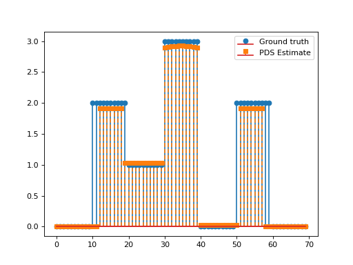
Consider the following optimisation problem:
\[\min_{\mathbf{x}\in\mathbb{R}_+^N}\frac{1}{2}\left\|\mathbf{y}-\mathbf{G}\mathbf{x}\right\|_2^2\quad+\quad\lambda_1 \|\mathbf{D}\mathbf{x}\|_1\quad+\quad\lambda_2 \|\mathbf{x}\|_1,\]
with \(\mathbf{D}\in\mathbb{R}^{N\times N}\) the discrete derivative operator and \(\mathbf{G}\in\mathbb{R}^{L\times N}, \, \mathbf{y}\in\mathbb{R}^L, \lambda_1,\lambda_2>0.\)
This problem can be solved via the PrimalDualSplitting algorithm with \(\mathcal{F}(\mathbf{x})= \frac{1}{2}\left\|\mathbf{y}-\mathbf{G}\mathbf{x}\right\|_2^2\), \(\mathcal{G}(\mathbf{x})=\lambda_2\|\mathbf{x}\|_1,\)
\(\mathcal{H}(\mathbf{x})=\lambda \|\mathbf{x}\|_1\) and \(\mathbf{K}=\mathbf{D}\).
import numpy as np
import matplotlib.pyplot as plt
from pycsou.linop.diff import FirstDerivative
from pycsou.func.loss import SquaredL2Loss
from pycsou.func.penalty import L1Norm, NonNegativeOrthant
from pycsou.linop.sampling import DownSampling
from pycsou.opt.proxalgs import PrimalDualSplitting

x = np.repeat([0, 2, 1, 3, 0, 2, 0], 10)
D = FirstDerivative(size=x.size, kind='forward')
D.compute_lipschitz_cst(tol=1e-3)
rng = np.random.default_rng(0)
Gop = DownSampling(size=x.size, downsampling_factor=3)
Gop.compute_lipschitz_cst()
y = Gop(x)
l22_loss = (1 / 2) * SquaredL2Loss(dim=Gop.shape[0], data=y)
F = l22_loss * Gop
lambda_ = 0.1
H = lambda_ * L1Norm(dim=D.shape[0])
G = 0.01 * L1Norm(dim=Gop.shape[1])
pds = PrimalDualSplitting(dim=Gop.shape[1], F=F, G=G, H=H, K=D, verbose=None)
estimate, converged, diagnostics = pds.iterate()
plt.figure()
plt.stem(x, linefmt='C0-', markerfmt='C0o')
plt.stem(estimate['primal_variable'], linefmt='C1--', markerfmt='C1s')
plt.legend(['Ground truth', 'PDS Estimate'])
plt.show()
(Source code, png, hires.png, pdf)
LASSO
Consider the LASSO problem:
\[\min_{\mathbf{x}\in\mathbb{R}^N}\frac{1}{2}\left\|\mathbf{y}-\mathbf{G}\mathbf{x}\right\|_2^2\quad+\quad\lambda \|\mathbf{x}\|_1,\]
with \(\mathbf{G}\in\mathbb{R}^{L\times N}, \, \mathbf{y}\in\mathbb{R}^L, \lambda>0.\) This problem can be solved via APGD with \(\mathcal{F}(\mathbf{x})= \frac{1}{2}\left\|\mathbf{y}-\mathbf{G}\mathbf{x}\right\|_2^2\) and \(\mathcal{G}(\mathbf{x})=\lambda \|\mathbf{x}\|_1\). We have:
\[\mathbf{\nabla}\mathcal{F}(\mathbf{x})=\mathbf{G}^T(\mathbf{G}\mathbf{x}-\mathbf{y}), \qquad \text{prox}_{\lambda\|\cdot\|_1}(\mathbf{x})=\text{soft}_\lambda(\mathbf{x}).\]
This yields the so-called Fast Iterative Soft Thresholding Algorithm (FISTA), whose convergence is guaranteed for \(d>2\) and \(0<\tau\leq \beta^{-1}=\|\mathbf{G}\|_2^{-2}\).
import numpy as np import matplotlib.pyplot as plt from pycsou.func.loss import SquaredL2Loss from pycsou.func.penalty import L1Norm from pycsou.linop.base import DenseLinearOperator from pycsou.opt.proxalgs import APGD rng = np.random.default_rng(0) Gop = DenseLinearOperator(rng.standard_normal(15).reshape(3,5)) Gop.compute_lipschitz_cst() x = np.zeros(Gop.shape[1]) x[1] = 1 x[-2] = -1 y = Gop(x) l22_loss = (1/2) * SquaredL2Loss(dim=Gop.shape[0], data=y) F = l22_loss * Gop lambda_ = 0.9 * np.max(np.abs(F.gradient(0 * x))) G = lambda_ * L1Norm(dim=Gop.shape[1]) apgd = APGD(dim=Gop.shape[1], F=F, G=G, acceleration='CD', verbose=None) estimate, converged, diagnostics = apgd.iterate() plt.figure() plt.stem(x, linefmt='C0-', markerfmt='C0o') plt.stem(estimate['iterand'], linefmt='C1--', markerfmt='C1s') plt.legend(['Ground truth', 'LASSO Estimate']) plt.show()(Source code, png, hires.png, pdf)
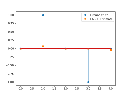