Background Concepts
Data Model
Most real-life approximation problems can be formulated as inverse problems.
Note
Consider an unknown signal \(f\in \mathcal{L}^2\left(\mathbb{R}^d\right)\) and assume that the latter is probed by some sensing device, resulting in a data vector \(\mathbf{y}=[y_1,\ldots,y_L]\in\mathbb{R}^L\) of \(L\) measurements. Recovering \(f\) from the data vector \(\mathbf{y}\) is called an inverse problem.
The following assumptions are standard:
To account for sensing inaccuracies, the data vector \(\mathbf{y}\) is assumed to be the outcome of a random vector \(\mathbf{Y}=[Y_1,\ldots,Y_L]:\Omega\rightarrow \mathbb{R}^L\), fluctuating according to some noise distribution. The entries of \(\mathbb{E}[\mathbf{Y}]=\tilde{\mathbf{y}}\) are called the ideal measurements –these are the measurements that would be obtained in the absence of noise.
The measurements are assumed unbiased and linear, i.e. \(\mathbb{E}[\mathbf{Y}]=\Phi^\ast f=\left[\langle f, \varphi_1\rangle, \ldots, \langle f,\varphi_L\rangle\right],\) for some sampling functionals \(\{\varphi_1,\ldots,\varphi_L\}\subset \mathcal{L}^2\left(\mathbb{R}^d\right)\), modelling the acquisition system.
See also
See Linear Operators for common sampling functionals provided by Pycsou (spatial sampling, subsampling, Fourier/Radon sampling, filtering, mean-pooling, etc…)
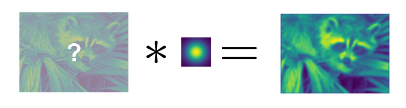
Image deblurring is a common example of inverse problem.
Discretisation
Since the number of measurements is finite, it is reasonable to constrain the signal \(f\) to be finite-dimensional:1
for some suitable basis functions \(\{\psi_n, \,n=1,\ldots,N\}\subset\mathcal{L}^2(\mathbb{R}^d)\). Typically, the basis functions are chosen as indicator functions of regular rectangular tiles of \(\mathbb{R}^d\) called pixels. For example:
where \(\mathbf{c}=[c_1,\ldots,c_d]\) are the coordinates of the lower-left corner of the first pixel, and \(\{h_1,\ldots,h_d\}\) are the sizes of the pixels across each dimension. The parametric signal \(f\) is then a piecewise constant signal than can be stored/manipulated/displayed efficiently via multi-dimensional array (hence the popularity of pixel-based discretisation schemes).
Example of a pixelated signal.
Note
Other popular choices of basis functions include: sines/cosines, radial basis functions, splines, polynomials…
Pixelisation induces a discrete inverse problem:
Find \(\mathbf{\alpha}\in\mathbb{R}^N\) from the noisy measurements \(\mathbf{y}\sim \mathbf{Y}\) where \(\mathbb{E}[\mathbf{Y}]=\mathbf{G}\mathbf{\alpha}\).
The operator \(\mathbf{G}:\mathbb{R}^N\to \mathbb{R}^L\) is a rectangular matrix given by:2
where \(\eta=\Pi_{k=1}^d h_k\), and \(\{\Omega_n\}_{n} \subset\mathcal{P}(\mathbb{R}^d)\) and \(\{\mathbf{\xi}_n\}_n\subset\mathbb{R}^d\) are the supports and centroids of each pixel, respectively.
Inverse Problems are Ill-Posed
To solve the inverse problem one can approximate the mean \(\mathbb{E}[Y]\) by its one-sample empirical estimate \(\mathbf{y}\) and solve the linear problem:
Unfortunately, such problems are in general ill-posed:
There may exist no solutions. If \(\mathbf{G}\) is not surjective, \(\mathcal{R}(\mathbf{G})\subsetneq \mathbb{R}^L\). Therefore the noisy data vector \(\mathbf{y}\) is not guaranteed to belong to \(\mathcal{R}(\mathbf{G})\).
There may exist more than one solution. If \(L<N\) indeed (or more generally if \(\mathbf{G}\) is not injective), \(\mathcal{N}(\mathbf{G})\neq \{\mathbf{0}\}\). Therefore, if \(\mathbf{\alpha}^\star\) is a solution to eqref{inverse_pb_linear_system}, then \(\mathbf{\alpha}^\star + \mathbf{\beta}\) is also a solution \(\forall\mathbf{\beta}\in \mathcal{N}(\mathbf{G})\):
Solutions may be numerically unstable. If \(\mathbf{G}\) is surjective for example, then \(\mathbf{G}^\dagger=\mathbf{G}^T(\mathbf{G}\mathbf{G}^T)^{-1}\) is a right-inverse of \(\mathbf{G}\) and \(\mathbf{\alpha}^\star(\mathbf{y})=\mathbf{G}^T(\mathbf{G}\mathbf{G}^T)^{-1} \mathbf{y}\) is a solution to eqref{inverse_pb_linear_system}. We have then
The reconstruction linear map \(\mathbf{y}\mapsto \mathbf{\alpha}^\star(\mathbf{y})\) can hence be virtually unbounded making it unstable.
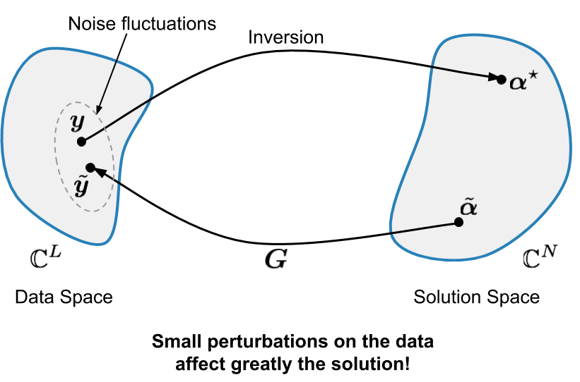
Inverse problems are unstable.
Regularising Inverse Problems
The linear system (1) is not only ill-posed but also non sensible: matching exactly the measurements is not desirable since the latter are in practice corrupted by instrumental noise.
A more sensible approach consists instead in solving the inverse problem by means of a penalised optimisation problem, confronting the physical evidence to the analyst’s a priori beliefs about the solution (e.g. smoothness, sparsity) via a data-fidelity and regularisation term, respectively:
The various quantities involved in the above equation can be interpreted as follows:
\(F:\mathbb{R}^L\times \mathbb{R}^L\rightarrow \mathbb{R}_+\cup\{+\infty\}\) is a cost/data-fidelity/loss functional, measuring the discrepancy between the observed and predicted measurements \(\mathbf{y}\) and \(\mathbf{G}\mathbf{\alpha}\) respectively.
\(\mathcal{R}:\mathbb{R}^N\to \mathbb{R}_+\cup\{+\infty\}\) is a regularisation/penalty functional favouring simple and well-behaved solutions (typically with a finite number of degrees of freedom).
\(\lambda>0\) is a regularisation/penalty parameter which controls the amount of regularisation by putting the regularisation functional and the cost functional on a similar scale.
Choosing the Loss Functional
The loss functional can be chosen as the negative log-likelihood of the data \(\mathbf{y}\):
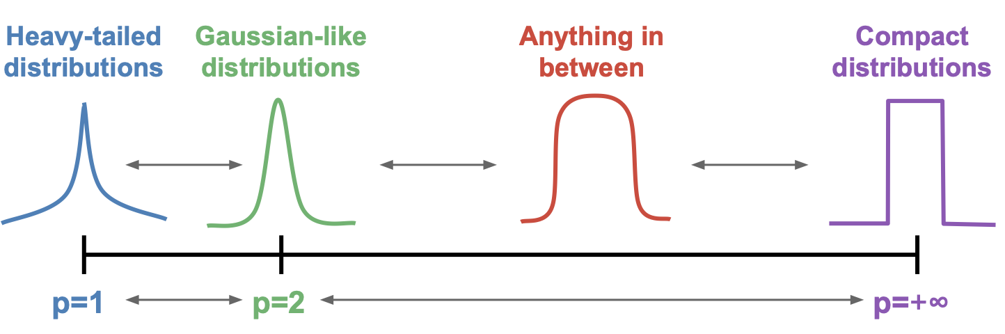
When the noise distribution is not fully known or the likelihood too complex, one can also use general \(\ell_p\) cost functionals
where \(p\in [1,+\infty]\) is typically chosen according to the tail behaviour of the noise distribution.
See also
See Loss Functionals for a rich collection of commonly used loss functionals provided by Pycsou.
Choosing the Penalty
The penalty/regularisation functional is used to favour physically-admissible solutions with simple behaviours. It can be interpreted as implementing Occam’s razor principle:
Occam’s razor principle is a philosophical principle also known as the law of briefness or in Latin lex parsimoniae. It was supposedly formulated by William of Ockham in the 14th century, who wrote in Latin Entia non sunt multiplicanda praeter necessitatem. In English, this translates to More things should not be used than are necessary.
In essence, this principle states that when two equally good explanations for a given phenomenon are available, one should always favour the simplest, i.e. the one that introduces the least explanatory variables. What exactly is meant by “simple” solutions will depend on the specific application at hand.
Common choices of regularisation strategies include: Tikhonov regularisation, TV regularisation, maximum entropy regularisation, etc…
See also
See Penalty Functionals for a rich collection of commonly used penalty functionals provided by Pycsou.
Proximal Algorithms
Most optimisation problems used to solve inverse problems in practice take the form:
where: * \(\mathcal{F}:\mathbb{R}^N\rightarrow \mathbb{R}\) is convex and differentiable, with \(\beta\)-Lipschitz continuous gradient. * \(\mathcal{G}:\mathbb{R}^N\rightarrow \mathbb{R}\cup\{+\infty\}\) and \(\mathcal{H}:\mathbb{R}^M\rightarrow \mathbb{R}\cup\{+\infty\}\) are two proper, lower semicontinuous and convex functions with simple proximal operators.
\(\mathbf{K}:\mathbb{R}^N\rightarrow \mathbb{R}^M\) is a linear operator.
Problems of the form (2) can be solved by means of iterative proximal algorithms:
Primal-dual splitting: solves for problems of the form \({\min_{\mathbf{x}\in\mathbb{R}^N} \mathcal{F}(\mathbf{x})+\mathcal{G}(\mathbf{x})+\mathcal{H}(\mathbf{K} \mathbf{x})}\)
Chambolle Pock splitting: solves for problems of the form \({\min_{\mathbf{x}\in\mathbb{R}^N} \mathcal{G}(\mathbf{x})+\mathcal{H}(\mathbf{K} \mathbf{x})}\)
Douglas Rachford splitting/ADMM: solves for problems of the form \({\min_{\mathbf{x}\in\mathbb{R}^N} \mathcal{G}(\mathbf{x})+\mathcal{H}(\mathbf{x})}\)
Forward-Backward splitting/APGD: solves for problems of the form \(\min_{\mathbf{x}\in\mathbb{R}^N} \mathcal{F}(\mathbf{x})+\mathcal{G}(\mathbf{x})\)
These are all first-order algorithms: they rely only on the gradient of \(\mathcal{F}\), and/or the proximal operators of \(\mathcal{G}, \mathcal{H}\), and/or matrix/vector multiplications with \(\mathbf{K}\) and \(\mathbf{K}^T\).
See also
See Proximal Algorithms for implementations of the above mentionned algorithms in Pycsou.
Footnotes