Differential Operators
Module: pycsou.linop.diff
Discrete differential and integral operators.
This module provides differential operators for discrete signals defined over regular grids or arbitrary meshes (graphs).
Many of the linear operators provided in this module are derived from linear operators from PyLops.
1D Operators
|
First derivative. |
|
Second derivative. |
|
Generalised derivative. |
|
1D integral/cumsum operator. |
2D Operators
|
Gradient. |
|
Laplacian. |
|
Generalised Laplacian operator. |
|
First directional derivative. |
|
Second directional derivative. |
Directional gradient. |
|
|
Directional Laplacian. |
-
FirstDerivative(size: int, shape: Optional[tuple] = None, axis: int = 0, step: float = 1.0, edge: bool = True, dtype: str = 'float64', kind: str = 'forward') → pycsou.linop.base.PyLopLinearOperator[source]¶ First derivative.
This docstring was adapted from ``pylops.FirstDerivative``.
Approximates the first derivative of a multi-dimensional array along a specific
axisusing finite-differences.- Parameters
size (int) – Size of the input array.
shape (tuple) – Shape of the input array.
axis (int) – Axis along which to differentiate.
step (float) – Step size.
edge (bool) – For
kind='centered', use reduced order derivative at edges (True) or ignore them (False).dtype (str) – Type of elements in input array.
kind (str) – Derivative kind (
forward,centered, orbackward).
- Returns
First derivative operator.
- Return type
- Raises
ValueError – If
shapeandsizeare not compatible.NotImplementedError – If
kindis not one of:forward,centered, orbackward.
Examples
>>> x = np.repeat([0,2,1,3,0,2,0], 10)
>>> Dop = FirstDerivative(size=x.size)
>>> y = Dop * x
>>> np.sum(np.abs(y) > 0)
6
>>> np.allclose(y, np.diff(x, append=0))
True
import numpy as np
import matplotlib.pyplot as plt
from pycsou.linop.diff import FirstDerivative

x = np.repeat([0,2,1,3,0,2,0], 10)
Dop_bwd = FirstDerivative(size=x.size, kind='backward')
Dop_fwd = FirstDerivative(size=x.size, kind='forward')
Dop_cent = FirstDerivative(size=x.size, kind='centered')
y_bwd = Dop_bwd * x
y_cent = Dop_cent * x
y_fwd = Dop_fwd * x
plt.figure()
plt.plot(np.arange(x.size), x)
plt.plot(np.arange(x.size), y_bwd)
plt.plot(np.arange(x.size), y_cent)
plt.plot(np.arange(x.size), y_fwd)
plt.legend(['Signal', 'Backward', 'Centered', 'Forward'])
plt.title('First derivative')
plt.show()
(Source code, png, hires.png, pdf)
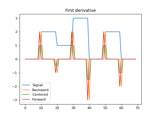
Notes
The
FirstDerivativeoperator applies a first derivative along a given axis of a multi-dimensional array using either a second-order centered stencil or first-order forward/backward stencils.For simplicity, given a one dimensional array, the second-order centered first derivative is:
\[y[i] = (0.5x[i+1] - 0.5x[i-1]) / \text{step}\]while the first-order forward stencil is:
\[y[i] = (x[i+1] - x[i]) / \text{step}\]and the first-order backward stencil is:
\[y[i] = (x[i] - x[i-1]) / \text{step}.\]See also
-
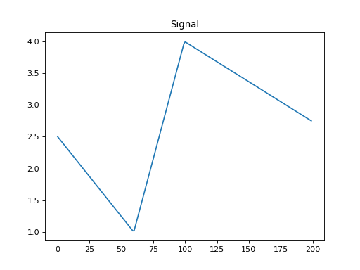
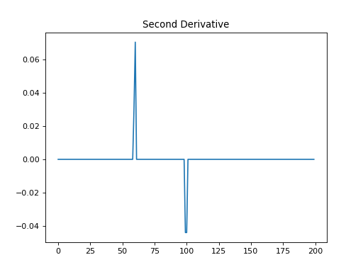
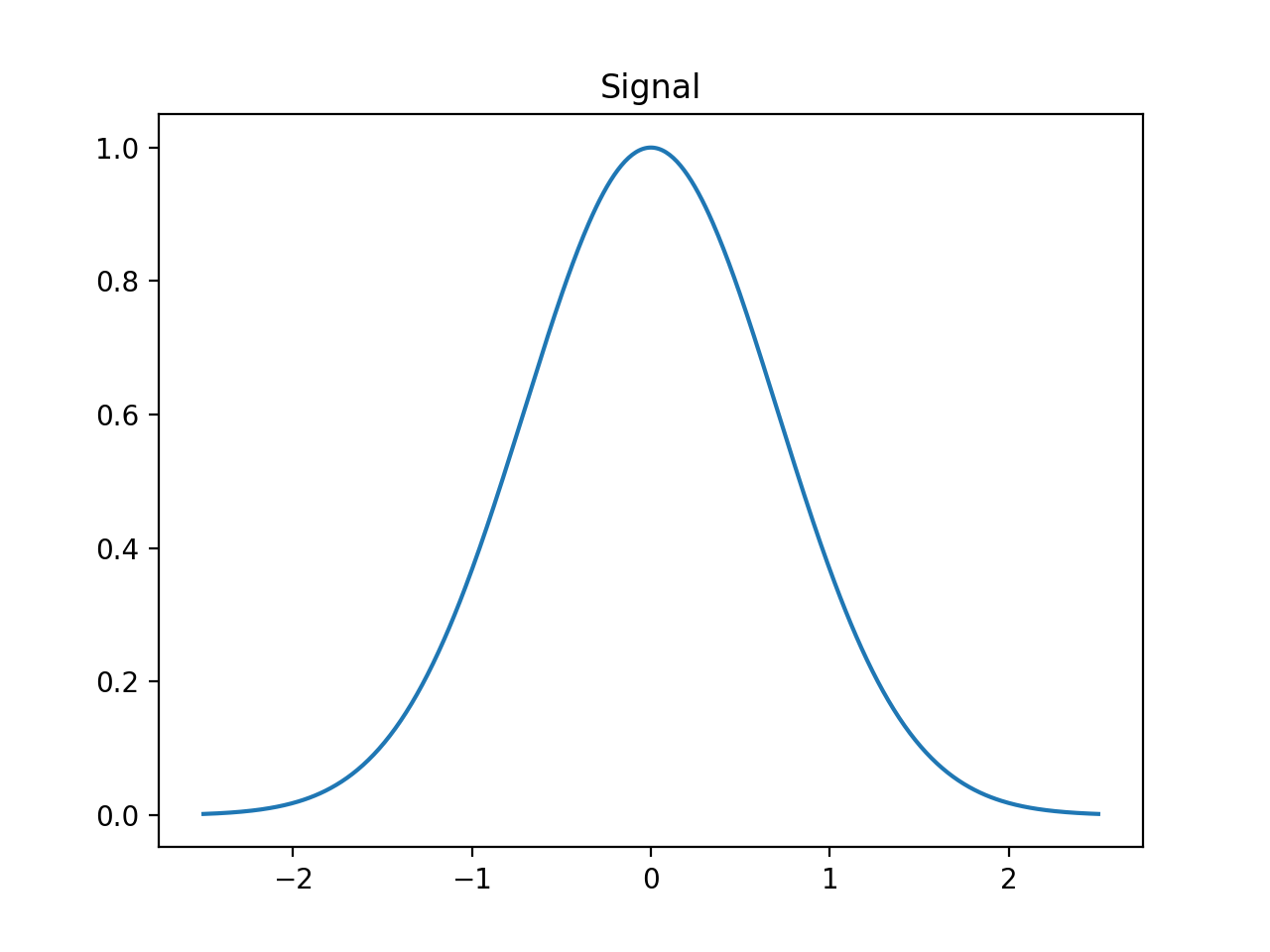
SecondDerivative(size: int, shape: Optional[tuple] = None, axis: int = 0, step: float = 1.0, edge: bool = True, dtype: str = 'float64') → pycsou.linop.base.PyLopLinearOperator[source]¶ Second derivative.
This docstring was adapted from ``pylops.SecondDerivative``.
Approximates the second derivative of a multi-dimensional array along a specific
axisusing finite-differences.- Parameters
- Returns
Second derivative operator.
- Return type
- Raises
ValueError – If
shapeandsizeare not compatible.
Examples
>>> x = np.linspace(-2.5, 2.5, 100)
>>> z = np.piecewise(x, [x < -1, (x >= - 1) * (x<0), x>=0], [lambda x: -x, lambda x: 3 * x + 4, lambda x: -0.5 * x + 4])
>>> Dop = SecondDerivative(size=x.size)
>>> y = Dop * z
import numpy as np
import matplotlib.pyplot as plt
from pycsou.linop.diff import SecondDerivative

x = np.linspace(-2.5, 2.5, 200)
z = np.piecewise(x, [x < -1, (x >= - 1) * (x<0), x>=0], [lambda x: -x, lambda x: 3 * x + 4, lambda x: -0.5 * x + 4])
Dop = SecondDerivative(size=x.size)
y = Dop * z
plt.figure()
plt.plot(np.arange(x.size), z)
plt.title('Signal')
plt.show()
(Source code, png, hires.png, pdf)
plt.figure()
plt.plot(np.arange(x.size), y)
plt.title('Second Derivative')
plt.show()

Notes
The
SecondDerivativeoperator applies a second derivative to any chosen direction of a multi-dimensional array.For simplicity, given a one dimensional array, the second-order centered second derivative is given by:
\[y[i] = (x[i+1] - 2x[i] + x[i-1]) / \text{step}^2.\]See also
-
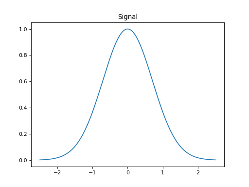
GeneralisedDerivative(size: int, shape: Optional[tuple] = None, axis: int = 0, step: float = 1.0, edge: bool = True, dtype: str = 'float64', kind_op='iterated', kind_diff='centered', **kwargs) → pycsou.core.linop.LinearOperator[source]¶ Generalised derivative.
Approximates the generalised derivative of a multi-dimensional array along a specific
axisusing finite-differences.- Parameters
size (int) – Size of the input array.
shape (tuple) – Shape of the input array.
axis (int) – Axis along which to differentiate.
step (float) – Step size.
edge (bool) – For
kind_diff = 'centered', use reduced order derivative at edges (True) or ignore them (False).dtype (str) – Type of elements in input array.
kind_diff (str) – Derivative kind (
forward,centered, orbackward).kind_op (str) –
Type of generalised derivative (
'iterated','sobolev','exponential','polynomial'). Depending on the cases, theGeneralisedDerivativeoperator is defined as follows:'iterated': \(\mathscr{D}=D^N\),'sobolev': \(\mathscr{D}=(\alpha^2 \mathrm{Id}-D^2)^N\), with \(\alpha\in\mathbb{R}\),'exponential': \(\mathscr{D}=(\alpha \mathrm{Id} + D)^N\), with \(\alpha\in\mathbb{R}\),'polynomial': \(\mathscr{D}=\sum_{n=0}^N \alpha_n D^n\), with \(\{\alpha_0,\ldots,\alpha_N\} \subset\mathbb{R}\),
where \(D\) is the
FirstDerivative()operator.kwargs (Any) –
Additional arguments depending on the value of
kind_op:'iterated':kwargs={order: int}whereorderdefines the exponent \(N\).'sobolev', 'exponential':kwargs={order: int, constant: float}whereorderdefines the exponent \(N\) andconstantthe scalar \(\alpha\in\mathbb{R}\).kind_op='polynomial':kwargs={coeffs: Union[np.ndarray, list, tuple]}wherecoeffsis an array containing the coefficients \(\{\alpha_0,\ldots,\alpha_N\} \subset\mathbb{R}\).
- Returns
A generalised derivative operator.
- Return type
- Raises
NotImplementedError – If
kind_opis not one of:'iterated','sobolev','exponential','polynomial'.
Examples
>>> x = np.linspace(-5, 5, 100)
>>> z = np.sinc(x)
>>> Dop = GeneralisedDerivative(size=x.size, kind_op='iterated', order=1, kind_diff='forward')
>>> D = FirstDerivative(size=x.size, kind='forward')
>>> np.allclose(Dop * z, D * z)
True
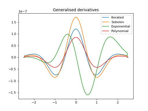
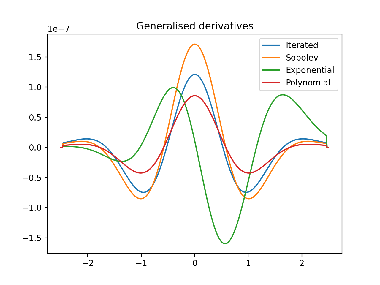
import numpy as np
import matplotlib.pyplot as plt
from pycsou.linop.diff import GeneralisedDerivative

x  = np.linspace(-2.5, 2.5, 500)
z = np.exp(-x ** 2)
Dop_it = GeneralisedDerivative(size=x.size, kind_op='iterated', order=4)
Dop_sob = GeneralisedDerivative(size=x.size, kind_op='sobolev', order=2, constant=1e-2)
Dop_exp = GeneralisedDerivative(size=x.size, kind_op='exponential', order=4, constant=-1e-2)
Dop_pol = GeneralisedDerivative(size=x.size, kind_op='polynomial',
                                coeffs= 1/2 * np.array([1e-8, 0, -2 * 1e-4, 0, 1]))
y_it = Dop_it * z
y_sob = Dop_sob * z
y_exp = Dop_exp * z
y_pol = Dop_pol * z
plt.figure()
plt.plot(x, z)
plt.title('Signal')
plt.show()
(Source code, png, hires.png, pdf)
plt.figure()
plt.plot(x, y_it)
plt.plot(x, y_sob)
plt.plot(x, y_exp)
plt.plot(x, y_pol)
plt.legend(['Iterated', 'Sobolev', 'Exponential', 'Polynomial'])
plt.title('Generalised derivatives')
plt.show()

Notes
Problematic values at edges are set to zero.
-
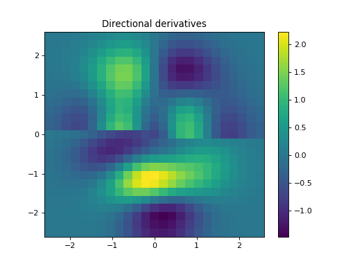
FirstDirectionalDerivative(shape: tuple, directions: numpy.ndarray, step: Union[float, Tuple[float, ...]] = 1.0, edge: bool = True, dtype: str = 'float64', kind: str = 'centered') → pycsou.linop.base.PyLopLinearOperator[source]¶ First directional derivative.
Computes the directional derivative of a multi-dimensional array (at least two dimensions are required) along either a single common direction or different
directionsfor each entry of the array.- Parameters
shape (tuple) – Shape of the input array.
directions (np.ndarray) – Single direction (array of size \(n_{dims}\)) or different directions for each entry (array of size \([n_{dims} \times (n_{d_0} \times ... \times n_{d_{n_{dims}}})]\)). Each column should be normalised.
step (Union[float, Tuple[float, ..]]) – Step size in each direction.
edge (bool) – For
kind = 'centered', use reduced order derivative at edges (True) or ignore them (False).dtype (str) – Type of elements in input vector.
kind (str) – Derivative kind (
forward,centered, orbackward).
- Returns
Directional derivative operator.
- Return type
Examples
>>> x = np.linspace(-2.5, 2.5, 100)
>>> X,Y = np.meshgrid(x,x)
>>> Z = peaks(X, Y)
>>> direction = np.array([1,0])
>>> Dop = FirstDirectionalDerivative(shape=Z.shape, directions=direction, kind='forward')
>>> D = FirstDerivative(size=Z.size, shape=Z.shape, kind='forward')
>>> np.allclose(Dop * Z.flatten(), D * Z.flatten())
True
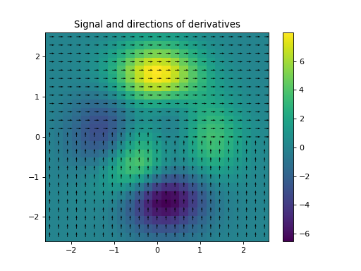
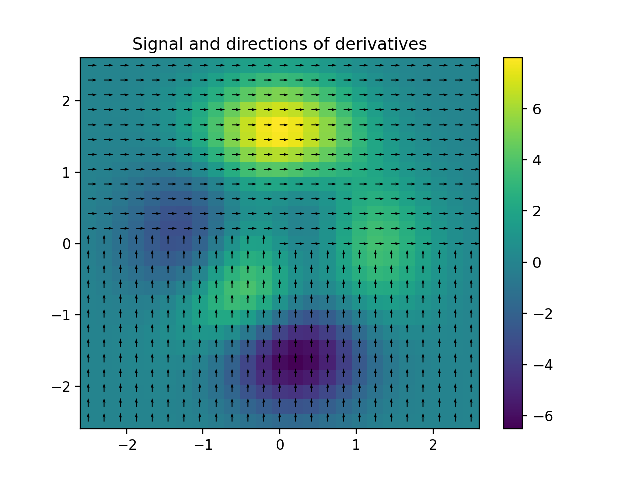
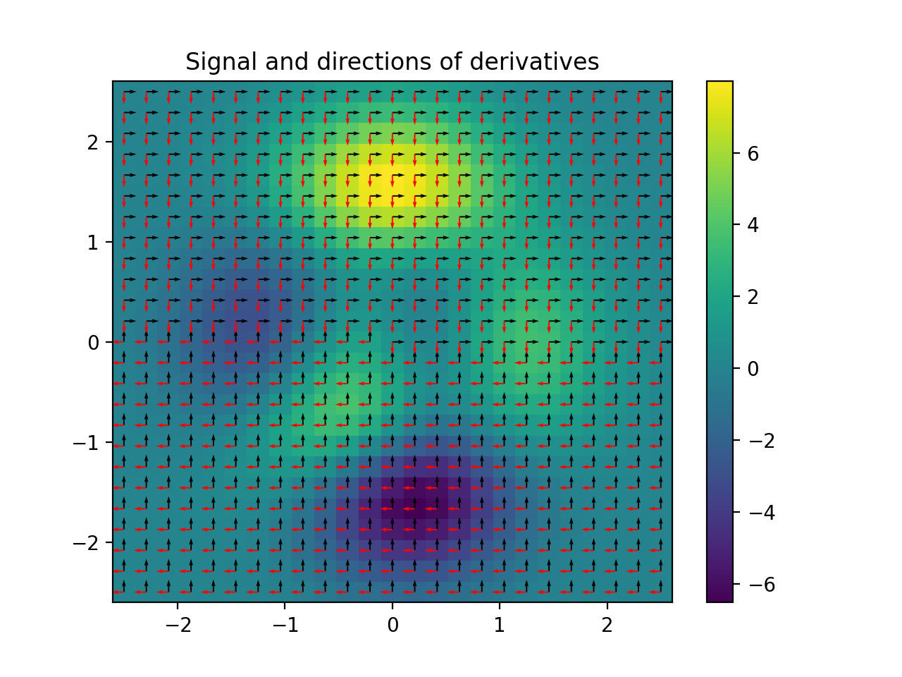
import numpy as np
import matplotlib.pyplot as plt
from pycsou.linop.diff import FirstDirectionalDerivative, FirstDerivative
from pycsou.util.misc import peaks

x  = np.linspace(-2.5, 2.5, 25)
X,Y = np.meshgrid(x,x)
Z = peaks(X, Y)
directions = np.zeros(shape=(2,Z.size))
directions[0, :Z.size//2] = 1
directions[1, Z.size//2:] = 1
Dop = FirstDirectionalDerivative(shape=Z.shape, directions=directions)
y = Dop * Z.flatten()

plt.figure()
h = plt.pcolormesh(X,Y,Z, shading='auto')
plt.quiver(x, x, directions[1].reshape(X.shape), directions[0].reshape(X.shape))
plt.colorbar(h)
plt.title('Signal and directions of derivatives')
plt.figure()
h = plt.pcolormesh(X,Y,y.reshape(X.shape), shading='auto')
plt.colorbar(h)
plt.title('Directional derivatives')
plt.show()
Notes
The
FirstDirectionalDerivativeapplies a first-order derivative to a multi-dimensional array along the direction defined by the unitary vector \(\mathbf{v}\):\[d_\mathbf{v}f = \langle\nabla f, \mathbf{v}\rangle,\]or along the directions defined by the unitary vectors \(\mathbf{v}(x, y)\):
\[d_\mathbf{v}(x,y) f = \langle\nabla f(x,y), \mathbf{v}(x,y)\rangle\]where we have here considered the 2-dimensional case. Note that the 2D case, choosing \(\mathbf{v}=[1,0]\) or \(\mathbf{v}=[0,1]\) is equivalent to the
FirstDerivativeoperator applied to axis 0 or 1 respectively.

-
SecondDirectionalDerivative(shape: tuple, directions: numpy.ndarray, step: Union[float, Tuple[float, ...]] = 1.0, edge: bool = True, dtype: str = 'float64')[source]¶ Second directional derivative.
Computes the second directional derivative of a multi-dimensional array (at least two dimensions are required) along either a single common direction or different
directionsfor each entry of the array.- Parameters
shape (tuple) – Shape of the input array.
directions (np.ndarray) – Single direction (array of size \(n_{dims}\)) or different directions for each entry (array of size \([n_{dims} \times (n_{d_0} \times ... \times n_{d_{n_{dims}}})]\)). Each column should be normalised.
step (Union[float, Tuple[float, ..]]) – Step size in each direction.
edge (bool) – Use reduced order derivative at edges (
True) or ignore them (False).dtype (str) – Type of elements in input vector.
- Returns
Second directional derivative operator.
- Return type
Examples
>>> x = np.linspace(-2.5, 2.5, 100)
>>> X,Y = np.meshgrid(x,x)
>>> Z = peaks(X, Y)
>>> direction = np.array([1,0])
>>> Dop = SecondDirectionalDerivative(shape=Z.shape, directions=direction)
>>> dir_d2 = (Dop * Z.reshape(-1)).reshape(Z.shape)
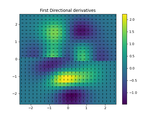
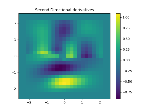
import numpy as np
import matplotlib.pyplot as plt
from pycsou.linop.diff import FirstDirectionalDerivative, SecondDirectionalDerivative
from pycsou.util.misc import peaks

x  = np.linspace(-2.5, 2.5, 25)
X,Y = np.meshgrid(x,x)
Z = peaks(X, Y)
directions = np.zeros(shape=(2,Z.size))
directions[0, :Z.size//2] = 1
directions[1, Z.size//2:] = 1
Dop = FirstDirectionalDerivative(shape=Z.shape, directions=directions)
Dop2 = SecondDirectionalDerivative(shape=Z.shape, directions=directions)
y = Dop * Z.flatten()
y2 = Dop2 * Z.flatten()

plt.figure()
h = plt.pcolormesh(X,Y,Z, shading='auto')
plt.quiver(x, x, directions[1].reshape(X.shape), directions[0].reshape(X.shape))
plt.colorbar(h)
plt.title('Signal and directions of derivatives')
plt.figure()
h = plt.pcolormesh(X,Y,y.reshape(X.shape), shading='auto')
plt.quiver(x, x, directions[1].reshape(X.shape), directions[0].reshape(X.shape))
plt.colorbar(h)
plt.title('First Directional derivatives')
plt.figure()
h = plt.pcolormesh(X,Y,y2.reshape(X.shape), shading='auto')
plt.colorbar(h)
plt.title('Second Directional derivatives')
plt.show()
Notes
The
SecondDirectionalDerivativeapplies a second-order derivative to a multi-dimensional array along the direction defined by the unitary vector \(\mathbf{v}\):\[d^2_\mathbf{v} f = - d_\mathbf{v}^\ast (d_\mathbf{v} f)\]where \(d_\mathbf{v}\) is the first-order directional derivative implemented by
FirstDirectionalDerivative(). The above formula generalises the well-known relationship:\[\Delta f= -\text{div}(\nabla f),\]where minus the divergence operator is the adjoint of the gradient.
Note that problematic values at edges are set to zero.

-
DirectionalGradient(first_directional_derivatives: List[pycsou.linop.diff.FirstDirectionalDerivative]) → pycsou.linop.base.LinOpVStack[source]¶ Directional gradient.
Computes the directional derivative of a multi-dimensional array (at least two dimensions are required) along multiple
directionsfor each entry of the array.- Parameters
first_directional_derivatives (List[FirstDirectionalDerivative]) – List of the directional derivatives to be stacked.
- Returns
Stack of first directional derivatives.
- Return type
Examples
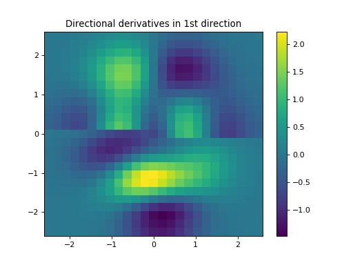
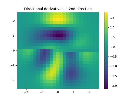
import numpy as np
import matplotlib.pyplot as plt
from pycsou.linop.diff import FirstDirectionalDerivative, DirectionalGradient
from pycsou.util.misc import peaks

x  = np.linspace(-2.5, 2.5, 25)
X,Y = np.meshgrid(x,x)
Z = peaks(X, Y)
directions1 = np.zeros(shape=(2,Z.size))
directions1[0, :Z.size//2] = 1
directions1[1, Z.size//2:] = 1
directions2 = np.zeros(shape=(2,Z.size))
directions2[1, :Z.size//2] = -1
directions2[0, Z.size//2:] = -1
Dop1 = FirstDirectionalDerivative(shape=Z.shape, directions=directions1)
Dop2 = FirstDirectionalDerivative(shape=Z.shape, directions=directions2)
Dop = DirectionalGradient([Dop1, Dop2])
y = Dop * Z.flatten()

plt.figure()
h = plt.pcolormesh(X,Y,Z, shading='auto')
plt.quiver(x, x, directions1[1].reshape(X.shape), directions1[0].reshape(X.shape))
plt.quiver(x, x, directions2[1].reshape(X.shape), directions2[0].reshape(X.shape), color='red')
plt.colorbar(h)
plt.title('Signal and directions of derivatives')
plt.figure()
h = plt.pcolormesh(X,Y,y[:Z.size].reshape(X.shape), shading='auto')
plt.colorbar(h)
plt.title('Directional derivatives in 1st direction')
plt.figure()
h = plt.pcolormesh(X,Y,y[Z.size:].reshape(X.shape), shading='auto')
plt.colorbar(h)
plt.title('Directional derivatives in 2nd direction')
plt.show()
Notes
The
DirectionalGradientof a multivariate function \(f(\mathbf{x})\) is defined as:\[\begin{split}d_{\mathbf{v}_1(\mathbf{x}),\ldots,\mathbf{v}_N(\mathbf{x})} f = \left[\begin{array}{c} \langle\nabla f, \mathbf{v}_1(\mathbf{x})\rangle\\ \vdots\\ \langle\nabla f, \mathbf{v}_N(\mathbf{x})\rangle \end{array}\right],\end{split}\]where \(d_\mathbf{v}\) is the first-order directional derivative implemented by
FirstDirectionalDerivative().See also

-
DirectionalLaplacian(second_directional_derivatives: List[pycsou.linop.diff.SecondDirectionalDerivative], weights: Optional[Iterable[float]] = None) → pycsou.core.linop.LinearOperator[source]¶ Directional Laplacian.
Sum of the second directional derivatives of a multi-dimensional array (at least two dimensions are required) along multiple
directionsfor each entry of the array.- Parameters
second_directional_derivatives (List[SecondDirectionalDerivative]) – List of the second directional derivatives to be summed.
weights (Optional[Iterable[float]]) – List of optional positive weights with which each second directional derivative operator is multiplied.
- Returns
Directional Laplacian.
- Return type
Examples
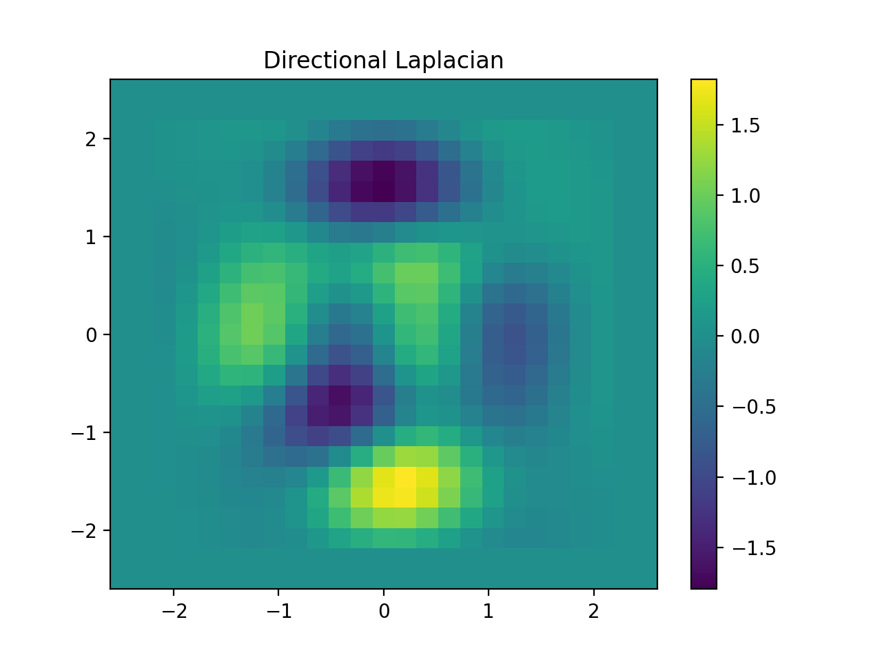
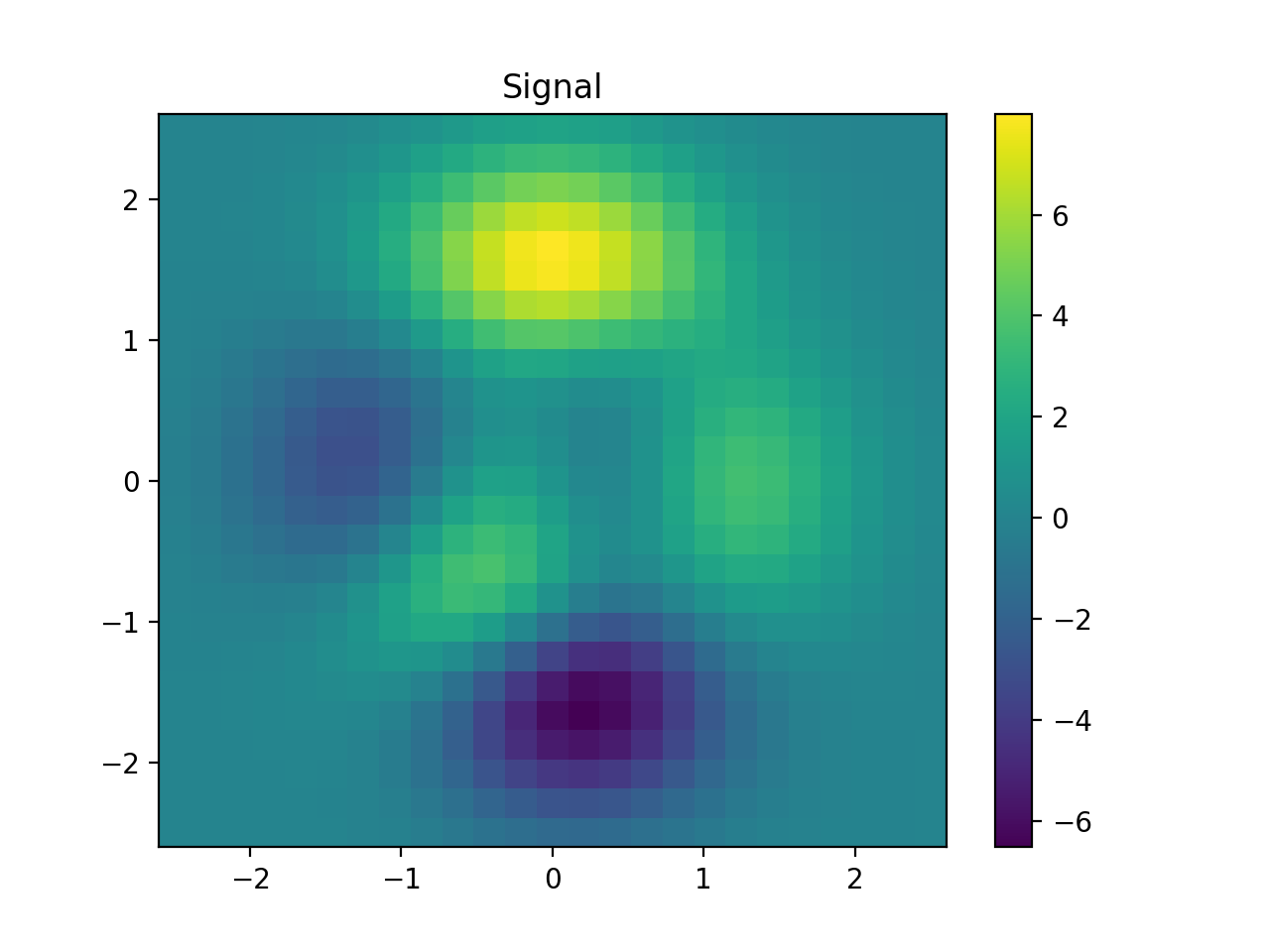
import numpy as np
import matplotlib.pyplot as plt
from pycsou.linop.diff import SecondDirectionalDerivative, DirectionalLaplacian
from pycsou.util.misc import peaks

x  = np.linspace(-2.5, 2.5, 25)
X,Y = np.meshgrid(x,x)
Z = peaks(X, Y)
directions1 = np.zeros(shape=(2,Z.size))
directions1[0, :Z.size//2] = 1
directions1[1, Z.size//2:] = 1
directions2 = np.zeros(shape=(2,Z.size))
directions2[1, :Z.size//2] = -1
directions2[0, Z.size//2:] = -1
Dop1 = SecondDirectionalDerivative(shape=Z.shape, directions=directions1)
Dop2 = SecondDirectionalDerivative(shape=Z.shape, directions=directions2)
Dop = DirectionalLaplacian([Dop1, Dop2])
y = Dop * Z.flatten()

plt.figure()
h = plt.pcolormesh(X,Y,Z, shading='auto')
plt.quiver(x, x, directions1[1].reshape(X.shape), directions1[0].reshape(X.shape))
plt.quiver(x, x, directions2[1].reshape(X.shape), directions2[0].reshape(X.shape), color='red')
plt.colorbar(h)
plt.title('Signal and directions of derivatives')
plt.figure()
h = plt.pcolormesh(X,Y,y.reshape(X.shape), shading='auto')
plt.colorbar(h)
plt.title('Directional Laplacian')
plt.show()
Notes
The
DirectionalLaplacianof a multivariate function \(f(\mathbf{x})\) is defined as:\[d^2_{\mathbf{v}_1(\mathbf{x}),\ldots,\mathbf{v}_N(\mathbf{x})} f = -\sum_{n=1}^N d^\ast_{\mathbf{v}_n(\mathbf{x})}(d_{\mathbf{v}_n(\mathbf{x})} f).\]where \(d_\mathbf{v}\) is the first-order directional derivative implemented by
FirstDirectionalDerivative().See also

-
Gradient(shape: tuple, step: Union[tuple, float] = 1.0, edge: bool = True, dtype: str = 'float64', kind: str = 'centered') → pycsou.linop.base.PyLopLinearOperator[source]¶ Gradient.
Computes the gradient of a multi-dimensional array (at least two dimensions are required).
- Parameters
shape (tuple) – Shape of the input array.
step (Union[float, Tuple[float, ..]]) – Step size in each direction.
edge (bool) – For
kind = 'centered', use reduced order derivative at edges (True) or ignore them (False).dtype (str) – Type of elements in input vector.
kind (str) – Derivative kind (
forward,centered, orbackward).
- Returns
Gradient operator.
- Return type
Examples
>>> x = np.linspace(-2.5, 2.5, 100)
>>> X,Y = np.meshgrid(x,x)
>>> Z = peaks(X, Y)
>>> Nabla = Gradient(shape=Z.shape, kind='forward')
>>> D = FirstDerivative(size=Z.size, shape=Z.shape, kind='forward')
>>> np.allclose((Nabla * Z.flatten())[:Z.size], D * Z.flatten())
True
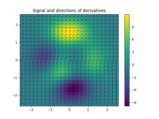
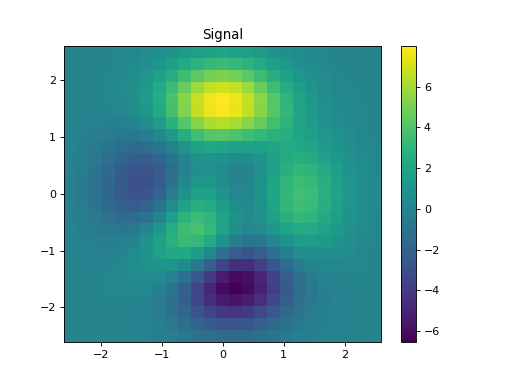
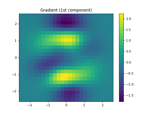
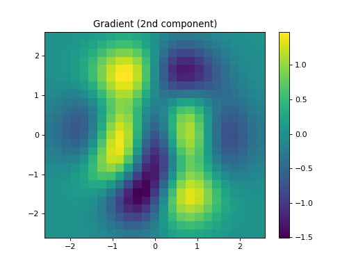
import numpy as np
import matplotlib.pyplot as plt
from pycsou.linop.diff import Gradient
from pycsou.util.misc import peaks

x  = np.linspace(-2.5, 2.5, 25)
X,Y = np.meshgrid(x,x)
Z = peaks(X, Y)
Dop = Gradient(shape=Z.shape)
y = Dop * Z.flatten()

plt.figure()
h = plt.pcolormesh(X,Y,Z, shading='auto')
plt.colorbar(h)
plt.title('Signal')
plt.figure()
h = plt.pcolormesh(X,Y,y[:Z.size].reshape(X.shape), shading='auto')
plt.colorbar(h)
plt.title('Gradient (1st component)')
plt.figure()
h = plt.pcolormesh(X,Y,y[Z.size:].reshape(X.shape), shading='auto')
plt.colorbar(h)
plt.title('Gradient (2nd component)')
plt.show()
Notes
The
Gradientoperator applies a first-order derivative to each dimension of a multi-dimensional array in forward mode.For simplicity, given a three dimensional array, the
Gradientin forward mode using a centered stencil can be expressed as:\[\mathbf{g}_{i, j, k} = (f_{i+1, j, k} - f_{i-1, j, k}) / d_1 \mathbf{i_1} + (f_{i, j+1, k} - f_{i, j-1, k}) / d_2 \mathbf{i_2} + (f_{i, j, k+1} - f_{i, j, k-1}) / d_3 \mathbf{i_3}\]which is discretized as follows:
\[\begin{split}\mathbf{g} = \begin{bmatrix} \mathbf{df_1} \\ \mathbf{df_2} \\ \mathbf{df_3} \end{bmatrix}.\end{split}\]In adjoint mode, the adjoints of the first derivatives along different axes are instead summed together.
See also
-
Laplacian(shape: tuple, weights: Tuple[float] = (1, 1), step: Union[tuple, float] = 1.0, edge: bool = True, dtype: str = 'float64') → pycsou.linop.base.PyLopLinearOperator[source]¶ Laplacian.
Computes the Laplacian of a 2D array.
- Parameters
shape (tuple) – Shape of the input array.
weights (Tuple[float]) – Weight to apply to each direction (real laplacian operator if
weights=[1,1])step (Union[float, Tuple[float, ..]]) – Step size in each direction.
edge (bool) – Use reduced order derivative at edges (
True) or ignore them (False).dtype (str) – Type of elements in input vector.
kind (str) – Derivative kind (
forward,centered, orbackward).
- Returns
Laplacian operator.
- Return type
Examples
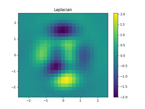
import numpy as np
import matplotlib.pyplot as plt
from pycsou.linop.diff import Laplacian
from pycsou.util.misc import peaks

x  = np.linspace(-2.5, 2.5, 25)
X,Y = np.meshgrid(x,x)
Z = peaks(X, Y)
Dop = Laplacian(shape=Z.shape)
y = Dop * Z.flatten()

plt.figure()
h = plt.pcolormesh(X,Y,Z, shading='auto')
plt.colorbar(h)
plt.title('Signal')
plt.figure()
h = plt.pcolormesh(X,Y,y.reshape(X.shape), shading='auto')
plt.colorbar(h)
plt.title('Laplacian')
plt.show()
Notes
The Laplacian operator sums the second directional derivatives of a 2D array along the two canonical directions.
It is defined as:
\[y[i, j] =\frac{x[i+1, j] + x[i-1, j] + x[i, j-1] +x[i, j+1] - 4x[i, j]} {dx\times dy}.\]See also

-
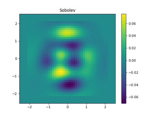
GeneralisedLaplacian(shape: Optional[tuple] = None, step: Union[tuple, float] = 1.0, edge: bool = True, dtype: str = 'float64', kind='iterated', **kwargs) → pycsou.core.linop.LinearOperator[source]¶ Generalised Laplacian operator.
Generalised Laplacian operator for a 2D array.
- Parameters
shape (tuple) – Shape of the input array.
step (Union[tuple, float] = 1.) – Step size for each dimension.
edge (bool) – Use reduced order derivative at edges (
True) or ignore them (False).dtype (str) – Type of elements in input array.
kind (str) –
Type of generalised differential operator (
'iterated','sobolev','polynomial'). Depending on the cases, theGeneralisedLaplacianoperator is defined as follows:'iterated': \(\mathscr{D}=\Delta^N\),'sobolev': \(\mathscr{D}=(\alpha^2 \mathrm{Id}-\Delta)^N\), with \(\alpha\in\mathbb{R}\),'polynomial': \(\mathscr{D}=\sum_{n=0}^N \alpha_n \Delta^n\), with \(\{\alpha_0,\ldots,\alpha_N\} \subset\mathbb{R}\),
where \(\Delta\) is the
Laplacian()operator.kwargs (Any) –
Additional arguments depending on the value of
kind:'iterated':kwargs={order: int}whereorderdefines the exponent \(N\).'sobolev':kwargs={order: int, constant: float}whereorderdefines the exponent \(N\) andconstantthe scalar \(\alpha\in\mathbb{R}\).'polynomial':kwargs={coeffs: Union[np.ndarray, list, tuple]}wherecoeffsis an array containing the coefficients \(\{\alpha_0,\ldots,\alpha_N\} \subset\mathbb{R}\).
- Returns
Generalised Laplacian operator.
- Return type
- Raises
NotImplementedError – If
kindis not one of:'iterated','sobolev','polynomial'.
Examples
import numpy as np
import matplotlib.pyplot as plt
from pycsou.linop.diff import GeneralisedLaplacian
from pycsou.util.misc import peaks

x  = np.linspace(-2.5, 2.5, 50)
X,Y = np.meshgrid(x,x)
Z = peaks(X, Y)
Dop = GeneralisedLaplacian(shape=Z.shape, kind='sobolev', order=2, constant=0)
y = Dop * Z.flatten()

plt.figure()
h = plt.pcolormesh(X,Y,Z, shading='auto')
plt.colorbar(h)
plt.title('Signal')
plt.figure()
h = plt.pcolormesh(X,Y,y.reshape(X.shape), shading='auto')
plt.colorbar(h)
plt.title('Sobolev')
plt.show()
Notes
Problematic values at edges are set to zero.
See also

-
Integration1D(size: int, shape: Optional[tuple] = None, axis: int = 0, step: float = 1.0, dtype='float64') → pycsou.linop.base.PyLopLinearOperator[source]¶ 1D integral/cumsum operator.
Integrates a multi-dimensional array along a specific
axis.- Parameters
- Returns
Integral operator.
- Return type
Examples
import numpy as np
import matplotlib.pyplot as plt
from pycsou.linop.diff import Integration1D

x = np.array([0,0,0,1,0,0,0,0,0,2,0,0,0,0,-1,0,0,0,0,2,0,0,0,0])
Int = Integration1D(size=x.size)
y = Int * x
plt.figure()
plt.plot(np.arange(x.size), x)
plt.plot(np.arange(x.size), y)
plt.legend(['Signal', 'Integral'])
plt.title('Integration')
plt.show()
(Source code, png, hires.png, pdf)
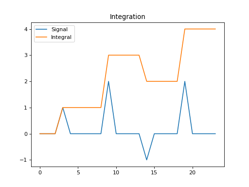
Notes
The
Integration1Doperator applies a causal integration to any chosen direction of a multi-dimensional array.For simplicity, given a one dimensional array, the causal integration is:
\[y(t) = \int x(t) dt\]which can be discretised as :
\[y[i] = \sum_{j=0}^i x[j] dt,\]where \(dt\) is the
samplinginterval.See also