Sampling Operators¶

Module: pycsou.linop.sampling

Sampling operators.

This module provides sampling operators for discrete or continuous signals.

Discrete Sampling Operators

`SubSampling`(size, sampling_indices[, shape, …])	Subsampling operator.
`Masking`(size, sampling_bool[, dtype])	Masking operator.
`DownSampling`(size, downsampling_factor[, …])	Downsampling operator.
`Pooling`(shape, block_size[, pooling_func, dtype])	Pooling operator.

Continuous-Domain Sampling Operators

`NNSampling`(samples, grid[, dtype])	Nearest neighbours sampling operator.
`GeneralisedVandermonde`(samples, funcs[, dtype])	Generalised Vandermonde matrix.
`MappedDistanceMatrix`(samples1, function[, …])	Transformed Distance Matrix.

SubSampling(size: int, sampling_indices: Union[numpy.ndarray, list], shape: Optional[tuple] = None, axis: int = 0, dtype: str = 'float64', inplace: bool = True)[source]¶

Subsampling operator.

Extract subset of values from input array at locations sampling_indices in forward mode and place those values at locations sampling_indices in an otherwise zero array in adjoint mode.

Parameters

size (int) – Size of input array.
sampling_indices (list or numpy.ndarray) – Integer indices of samples for data selection.
shape (tuple) – Shape of input array (None if only one dimension is available).
axis (int) – When shape is not None, axis along which subsampling is applied.
dtype (str) – Type of elements in input array.
inplace (bool) – Work inplace (True) or make a new copy (False). By default, data is a reference to the model (in forward) and model is a reference to the data (in adjoint).

Returns

The subsampling operator.

Return type

PyLopLinearOperator

Raises

ValueError – If shape and size do not match.

Examples

>>> x = np.arange(9).reshape(3,3)
>>> sampling_indices = [0,2]
>>> SamplingOp=SubSampling(size=x.size, sampling_indices=sampling_indices)
>>> SamplingOp * x.reshape(-1)
array([0, 2])
>>> SamplingOp.adjoint(SamplingOp* x.reshape(-1)).reshape(x.shape)
array([[0., 0., 2.],
       [0., 0., 0.],
       [0., 0., 0.]])
>>> SamplingOp=SubSampling(size=x.size, sampling_indices=sampling_indices, shape=x.shape, axis=1)
>>> (SamplingOp * x.reshape(-1)).reshape(x.shape[1], len(sampling_indices))
array([[0, 2],
       [3, 5],
       [6, 8]])
>>> SamplingOp.adjoint(SamplingOp* x.reshape(-1)).reshape(x.shape)
array([[0., 0., 2.],
       [3., 0., 5.],
       [6., 0., 8.]])

Notes

Subsampling of a subset of \(L\) values at locations sampling_indices from an input vector \(\mathbf{x}\) of size \(N\) can be expressed as:

\[y_i = x_{n_i} \quad \forall i=1,2,...,L,\]

where \(\mathbf{n}=[n_1, n_2,..., n_L]\) is a vector containing the indeces of the original array at which samples are taken.

Conversely, in adjoint mode the available values in the data vector \(\mathbf{y}\) are placed at locations \(\mathbf{n}=[n_1, n_2,..., n_L]\) in the model vector:

\[x_{n_i} = y_i \quad \forall i=1,2,...,L\]

and \(x_{j}=0 \,\forall j \neq n_i\) (i.e., at all other locations in input vector).

See also

Masking, Downsampling

class Masking(size: int, sampling_bool: Union[numpy.ndarray, list], dtype: type = <class 'numpy.float64'>)[source]¶

Bases: pycsou.core.linop.LinearOperator

Masking operator.

Extract subset of values from input array at locations marked as True in sampling_bool.

Examples

>>> x = np.arange(9).reshape(3,3)
>>> sampling_bool = np.zeros((3,3)).astype(bool)
>>> sampling_bool[[1,2],[0,2]] = True
>>> SamplingOp = Masking(size=x.size, sampling_bool=sampling_bool)
>>> SamplingOp * x.reshape(-1)
array([3, 8])
>>> SamplingOp.adjoint(SamplingOp* x.reshape(-1)).reshape(x.shape)
array([[0., 0., 0.],
       [3., 0., 0.],
       [0., 0., 8.]])
>>> sampling_indices = np.nonzero(sampling_bool.reshape(-1))[0].astype(int)
>>> SubSamplingOp=SubSampling(size=x.size, sampling_indices=sampling_indices)
>>> np.allclose(SamplingOp * x.reshape(-1), SubSamplingOp * x.reshape(-1))
True

Notes

For flattened arrays, the Masking operator is equivalent to the SubSampling() operator, with the only difference that the sampling locations are specified in the form of a boolean array instead of indices.

See also

SubSampling, Downsampling

__init__(size: int, sampling_bool: Union[numpy.ndarray, list], dtype: type = <class 'numpy.float64'>)[source]¶

Parameters

size (int) – Size of input array.
sampling_bool (list or numpy.ndarray) – Boolean array for data selection. True values mark the positions of the samples.
dtype (str) –
of elements in input array. (Type) –

Raises

ValueError – If the size of sampling_bool differs from size.

adjoint(y: numpy.ndarray) → numpy.ndarray[source]¶

Evaluates the adjoint of the operator at a point.

Parameters: y (Union[Number, np.ndarray]) – Point at which the adjoint should be evaluated.
Returns: Evaluation of the adjoint at y.
Return type: Union[Number, np.ndarray]

class DownSampling(size: int, downsampling_factor: Union[int, tuple, list], shape: Optional[tuple] = None, axis: Optional[int] = None, dtype: type = <class 'numpy.float64'>)[source]¶

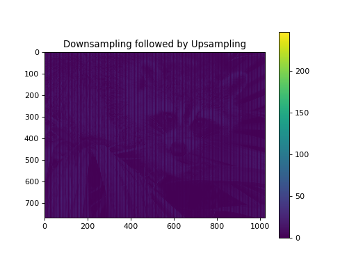
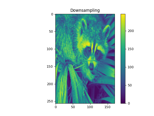
Bases: pycsou.linop.sampling.Masking

Downsampling operator.

Downsample an array in one of the three ways:

If shape is None: The input array is flat and the downsampling selects one element every downsampling_factor elements.
If shape is not None and axis is None: The input array is multidimensional, and each dimension is downsampled by a certain factor. Downsampling factors for each dimension are specified in the tuple downsampling_factor (if downsampling_factor is an integer, then the same factor is assumed for every dimension).
If shape is not None and axis is not None: The input array is multidimensional, but only the dimension is specified by axis is downsampled by a downsampling_factor.

Examples

>>> x = np.arange(10)
>>> DownSamplingOp = DownSampling(size=x.size, downsampling_factor=3)
>>> DownSamplingOp * x
array([0, 3, 6, 9])
>>> DownSamplingOp.adjoint(DownSamplingOp * x)
array([0., 0., 0., 3., 0., 0., 6., 0., 0., 9.])
>>> x = np.arange(20).reshape(4,5)
>>> DownSamplingOp = DownSampling(size=x.size, shape=x.shape, downsampling_factor=3)
>>> (DownSamplingOp * x.flatten()).reshape(DownSamplingOp.output_shape)
array([[ 0,  3],
       [15, 18]])
>>> DownSamplingOp = DownSampling(size=x.size, shape=x.shape, downsampling_factor=(2,4))
>>> (DownSamplingOp * x.flatten()).reshape(DownSamplingOp.output_shape)
array([[ 0,  4],
       [10, 14]])
>>> DownSamplingOp.adjoint(DownSamplingOp * x.flatten()).reshape(x.shape)
array([[ 0.,  0.,  0.,  0.,  4.],
       [ 0.,  0.,  0.,  0.,  0.],
       [10.,  0.,  0.,  0., 14.],
       [ 0.,  0.,  0.,  0.,  0.]])
>>> DownSamplingOp = DownSampling(size=x.size, shape=x.shape, downsampling_factor=2, axis=-1)
>>> (DownSamplingOp * x.flatten()).reshape(DownSamplingOp.output_shape)
array([[ 0,  2,  4],
       [ 5,  7,  9],
       [10, 12, 14],
       [15, 17, 19]])
>>> DownSamplingOp.adjoint(DownSamplingOp * x.flatten()).reshape(x.shape)
array([[ 0.,  0.,  2.,  0.,  4.],
       [ 5.,  0.,  7.,  0.,  9.],
       [10.,  0., 12.,  0., 14.],
       [15.,  0., 17.,  0., 19.]])

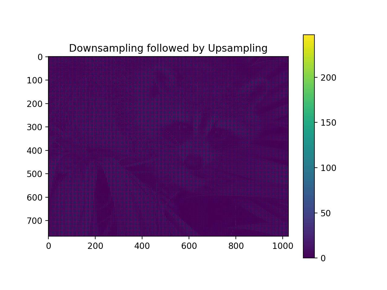
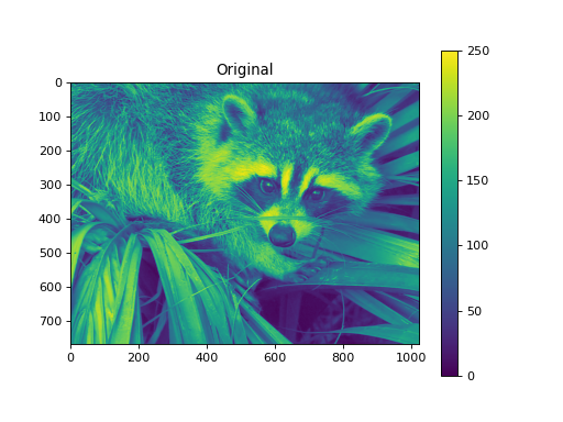
import numpy as np
from pycsou.linop.sampling import DownSampling
import matplotlib.pyplot as plt
import scipy.misc
img = scipy.misc.face(gray=True).astype(float)
DownSampOp = DownSampling(size=img.size, shape=img.shape, downsampling_factor=(3,6))
down_sampled_img = (DownSampOp * img.flatten()).reshape(DownSampOp.output_shape)
up_sampled_img = DownSampOp.adjoint(down_sampled_img.flatten()).reshape(img.shape)
plt.figure()
plt.imshow(img)
plt.colorbar()
plt.title('Original')
plt.figure()
plt.imshow(down_sampled_img)
plt.colorbar()
plt.title('Downsampling')
plt.figure()
plt.imshow(up_sampled_img)
plt.colorbar()
plt.title('Downsampling followed by Upsampling')

(Source code)

../../_images/pycsou-linop-sampling-1_00.png

(png, hires.png, pdf)¶

../../_images/pycsou-linop-sampling-1_01.png

(png, hires.png, pdf)¶

../../_images/pycsou-linop-sampling-1_02.png

(png, hires.png, pdf)¶

Notes

Downsampling by \(M\) an input vector \(\mathbf{x}\) of size \(N\) can be performed as:

\[y_i = x_{iM} \quad i=1,\ldots, \lfloor N/M \rfloor.\]

Conversely, in adjoint mode the available values in the data vector \(\mathbf{y}\) are placed at locations \(n=iM\) in the model vector:

\[x_{iM} = y_i,\;\;x_{iM+1}=x_{iM+2}=\cdots=x_{(i+1)M-1}=0, \qquad i=1,\ldots, \lfloor N/M \rfloor.\]

See also

SubSampling, Masking

__init__(size: int, downsampling_factor: Union[int, tuple, list], shape: Optional[tuple] = None, axis: Optional[int] = None, dtype: type = <class 'numpy.float64'>)[source]¶

Parameters

size (int) – Size of input array.
downsampling_factor (Union[int, tuple, list]) – Downsampling factor (possibly different for each dimension).
shape (Optional[tuple]) – Shape of input array (default None: the input array is 1D).
axis (Optional[int]) – Axis along which to downsample for ND input arrays (default None: downsampling is performed along each axis).
dtype (type) – Type of input array.

Raises

ValueError – If the set of parameters {shape, size, sampling_factor, axis} is invalid.

compute_downsampling_mask() → numpy.ndarray[source]¶

Compute the downsampling mask.

Returns: The mask to apply to get the downsampled values.
Return type: np.ndarray

class Pooling(shape: tuple, block_size: Union[tuple, list], pooling_func: str = 'mean', dtype: type = <class 'numpy.float64'>)[source]¶

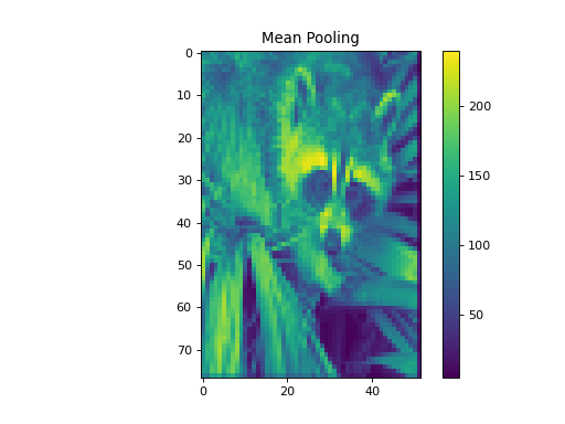
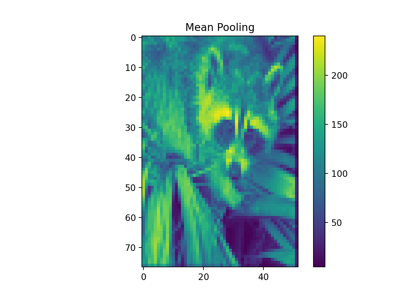
Bases: pycsou.core.linop.LinearOperator

Pooling operator.

Pool an array by summing/averaging across constant size blocks tiling the array.

Examples

>>> x = np.arange(24).reshape(4,6)
>>> PoolingOp = Pooling(shape=x.shape, block_size=(2,3), pooling_func='mean')
>>> (PoolingOp * x.flatten()).reshape(PoolingOp.output_shape)
array([[ 4.,  7.],
       [16., 19.]])
>>> PoolingOp.adjoint(PoolingOp * x.flatten()).reshape(x.shape)
array([[ 4.,  4.,  4.,  7.,  7.,  7.],
       [ 4.,  4.,  4.,  7.,  7.,  7.],
       [16., 16., 16., 19., 19., 19.],
       [16., 16., 16., 19., 19., 19.]])
>>> PoolingOp = Pooling(shape=x.shape, block_size=(2,3), pooling_func='sum')
>>> (PoolingOp * x.flatten()).reshape(PoolingOp.output_shape)
array([[ 24,  42],
       [ 96, 114]])
>>> PoolingOp.adjoint(PoolingOp * x.flatten()).reshape(x.shape)
array([[ 24,  24,  24,  42,  42,  42],
       [ 24,  24,  24,  42,  42,  42],
       [ 96,  96,  96, 114, 114, 114],
       [ 96,  96,  96, 114, 114, 114]])

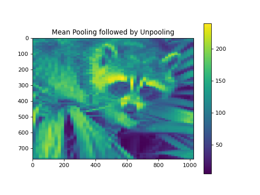
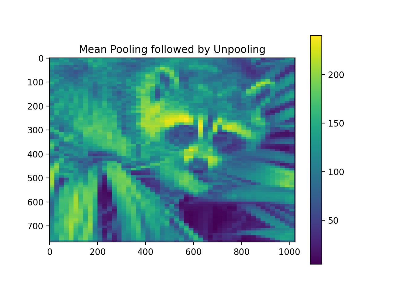
import numpy as np
from pycsou.linop.sampling import Pooling
import matplotlib.pyplot as plt
import scipy.misc
img = scipy.misc.face(gray=True).astype(float)
PoolingOp = Pooling(shape=img.shape, block_size=(10,20))
pooled_img = (PoolingOp * img.flatten()).reshape(PoolingOp.output_shape)
adjoint_img = PoolingOp.adjoint(pooled_img.flatten()).reshape(img.shape)
plt.figure()
plt.imshow(img)
plt.colorbar()
plt.title('Original')
plt.figure()
plt.imshow(pooled_img)
plt.colorbar()
plt.title('Mean Pooling')
plt.figure()
plt.imshow(adjoint_img)
plt.colorbar()
plt.title('Mean Pooling followed by Unpooling')

(Source code)

../../_images/pycsou-linop-sampling-2_00.png

(png, hires.png, pdf)¶

../../_images/pycsou-linop-sampling-2_01.png

(png, hires.png, pdf)¶

../../_images/pycsou-linop-sampling-2_02.png

(png, hires.png, pdf)¶

Notes

Pooling is performed via the function skimage.measure.block_reduce from scikit-image. If one dimension of the image is not perfectly divisible by the block size then it is zero padded.

The adjoint (unpooling) is performed by assigning the value of the blocks through the pooling function (e.g. mean, sum) to each element of the blocks.

Warning

Max, median or min pooling are not supported since the resulting PoolingOperator would then be non linear!

See also

SubSampling, Downsampling

__init__(shape: tuple, block_size: Union[tuple, list], pooling_func: str = 'mean', dtype: type = <class 'numpy.float64'>)[source]¶

Parameters

shape (tuple) – Shape of the input array.
block_size (Union[tuple, list]) – Shape of the sub-blocks on which pooling is performed.
pooling_func (str) – Specifies if the local blocks should be summed (pooling_func=’sum’) or averaged (pooling_func=’mean’).
dtype – Type of input array.

Raises

ValueError – If the block size is inconsistent with the input array shape or if the pooling function is not supported.

get_output_shape() → tuple[source]¶

Get shape of the pooled array.

Returns: Output array shape.
Return type: tuple

adjoint(y: numpy.ndarray) → numpy.ndarray[source]¶

Evaluates the adjoint of the operator at a point.

Parameters: y (Union[Number, np.ndarray]) – Point at which the adjoint should be evaluated.
Returns: Evaluation of the adjoint at y.
Return type: Union[Number, np.ndarray]

class NNSampling(samples: numpy.ndarray, grid: numpy.ndarray, dtype: type = <class 'numpy.float64'>)[source]¶

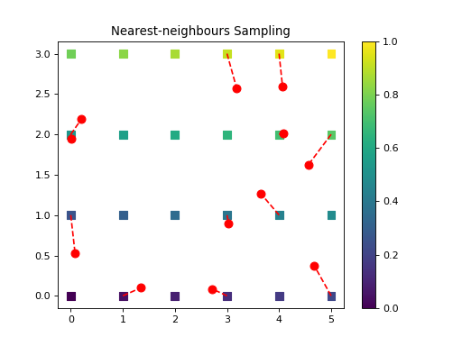
Bases: pycsou.core.linop.LinearOperator

Nearest neighbours sampling operator.

Sample a gridded ND signal at on-grid nearest neighbours of off-grid sampling locations. This can be useful when piecewise constant priors are used to recover continuously-defined signals sampled non-uniformly (see [FuncSphere] Remark 6.9).

Examples

>>> rng = np.random.default_rng(seed=0)
>>> x = np.arange(24).reshape(4,6)
>>> grid = np.stack(np.meshgrid(np.arange(6),np.arange(4)), axis=-1)
>>> samples = np.stack((5 * rng.random(size=6),3 * rng.random(size=6)), axis=-1)
>>> print(samples)
[[3.18480844 1.81990733]
 [1.34893357 2.18848968]
 [0.20486762 1.63087497]
 [0.08263818 2.80521727]
 [4.0663512  2.44756066]
 [4.56377789 0.0082155 ]]
>>> NNSamplingOp = NNSampling(samples=samples, grid=grid)
>>> (NNSamplingOp * x.flatten())
array([15, 13, 12, 18, 16,  5])
>>> NNSamplingOp.adjoint(NNSamplingOp * x.flatten()).reshape(x.shape)
array([[ 0.,  0.,  0.,  0.,  0.,  5.],
       [ 0.,  0.,  0.,  0.,  0.,  0.],
       [12., 13.,  0., 15., 16.,  0.],
       [18.,  0.,  0.,  0.,  0.,  0.]])

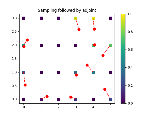
import numpy as np
from pycsou.linop.sampling import NNSampling
import matplotlib.pyplot as plt
rng = np.random.default_rng(seed=0)

rng = np.random.default_rng(seed=0)
x = np.arange(24).reshape(4, 6)
grid = np.stack(np.meshgrid(np.arange(6), np.arange(4)), axis=-1)
samples = np.stack((5 * rng.random(size=12), 3 * rng.random(size=12)), axis=-1)
NNSamplingOp = NNSampling(samples=samples, grid=grid)
grid = grid.reshape(-1, 2)
x = x.reshape(-1)
y = (NNSamplingOp * x.flatten())
x_samp = NNSamplingOp.adjoint(y).reshape(x.shape)
plt.scatter(grid[..., 0].reshape(-1), grid[..., 1].reshape(-1), s=64, c=x.reshape(-1), marker='s', vmin=np.min(x),
     vmax=np.max(x))
plt.scatter(samples[:, 0], samples[:, 1], c='r', s=64)
plt.plot(np.stack((grid[NNSamplingOp.nn_indices, 0], samples[:, 0]), axis=0),
  np.stack((grid[NNSamplingOp.nn_indices, 1], samples[:, 1]), axis=0), '--r')
plt.colorbar()
plt.title('Nearest-neighbours Sampling')
plt.figure()
plt.scatter(grid[..., 0].reshape(-1), grid[..., 1].reshape(-1), s=64, c=x_samp.reshape(-1), marker='s',
     vmin=np.min(x),
     vmax=np.max(x))
plt.scatter(samples[:, 0], samples[:, 1], c='r', s=64)
plt.plot(np.stack((grid[NNSamplingOp.nn_indices, 0], samples[:, 0]), axis=0),
  np.stack((grid[NNSamplingOp.nn_indices, 1], samples[:, 1]), axis=0), '--r')
plt.colorbar()
plt.title('Sampling followed by adjoint')

(Source code)

../../_images/pycsou-linop-sampling-3_00.png

(png, hires.png, pdf)¶

../../_images/pycsou-linop-sampling-3_01.png

(png, hires.png, pdf)¶

Notes

Consider a signal defined over a mesh \(f:\{\mathbf{n}_1,\ldots, \mathbf{n}_M\}\to \mathbb{C}\), with \(\{\mathbf{n}_1,\ldots, \mathbf{n}_M\}\subset \mathbb{R}^N\). Consider moreover sampling locations \(\{\mathbf{z}_1,\ldots, \mathbf{z}_L\}\subset \mathbb{R}^N\) which do not necessarily lie on the mesh. Then, nearest-neighbours sampling is defined as:

\[y_i=f\left[\arg\min_{k=1,\ldots, M}\|\mathbf{z}_i-\mathbf{n}_k\|_2\right], \qquad i=1,\ldots, L.\]

Note that in practice every sample locations has exactly one nearest neighbour (ties have probability zero) and hence this equation is well-defined.

Given a vector \(\mathbf{y}=[y_1,\ldots, y_L]\in\mathbb{C}^N\), the adjoint of the NNSampling operator is defined as

\[f[\mathbf{n}_k]=\mbox{mean}\left\{y_i :\; \mathbf{n}_k=\arg\min_{j=1,\ldots,M}\|\mathbf{z}_i-\mathbf{n}_j\|_2,\, i=1,\ldots, L\right\},\quad k=1,\ldots, M,\]

where \(\mbox{mean}\{B\}=|B|^{-1}\sum_{z\in B} z,\; \forall B\subset\mathbb{C}\) and with the convention that \(\mbox{mean}\{\emptyset\}=0.\) The mean is used to handle cases where many sampling locations are mapped to a common nearest neighbour on the mesh.

Warning

The grid needs not be uniform! Think of it as a mesh. It can happen that more than one sampling location is mapped to the same nearest neighbour.

See also

GeneralisedVandermonde

__init__(samples: numpy.ndarray, grid: numpy.ndarray, dtype: type = <class 'numpy.float64'>)[source]¶

Parameters

samples (np.ndarray) – Off-grid sampling locations with shape (M,N).
grid – Grid points with shape (L,N).
dtype (type) – Type of the input array.

Raises

ValueError – If the dimension of the sample locations and the grid points do not match.

compute_nn()[source]¶: Compute the on-grid nearest neighbours to the sampling locations.

adjoint(y: numpy.ndarray) → numpy.ndarray[source]¶

Evaluates the adjoint of the operator at a point.

Parameters: y (Union[Number, np.ndarray]) – Point at which the adjoint should be evaluated.
Returns: Evaluation of the adjoint at y.
Return type: Union[Number, np.ndarray]

class GeneralisedVandermonde(samples: numpy.ndarray, funcs: List[Callable], dtype: type = <class 'numpy.float64'>)[source]¶

Bases: pycsou.linop.base.DenseLinearOperator

Generalised Vandermonde matrix.

Given sampling locations \(\{\mathbf{z}_1,\ldots,\mathbf{z}_L\}\subset\mathbb{R}^N\), and a family of continuous functions \(\{\varphi_1, \ldots, \varphi_K\}\subset \mathcal{C}(\mathbb{R}^N, \mathbb{C})\), this function forms the generalised Vandermonde matrix:

\[\begin{split}\left[\begin{array}{ccc} \varphi_1(\mathbf{z}_1) & \cdots & \varphi_K(\mathbf{z}_1)\\\vdots & \ddots & \vdots\\\varphi_1(\mathbf{z}_L) & \cdots & \varphi_K(\mathbf{z}_L)\end{array}\right]\in\mathbb{C}^{L\times K}.\end{split}\]

This matrix is useful for sampling functions in the span of \(\{\varphi_1, \ldots, \varphi_K\}\). Indeed, if \(f=\sum_{k=1}^K\alpha_k\varphi_k\), then we have

\[\begin{split}\left[\begin{array}{c}f(\mathbf{z}_1)\\\vdots\\ f(\mathbf{z}_L) \end{array}\right]=\left[\begin{array}{ccc} \varphi_1(\mathbf{z}_1) & \cdots & \varphi_K(\mathbf{z}_1)\\\vdots & \ddots & \vdots\\\varphi_1(\mathbf{z}_L) & \cdots & \varphi_K(\mathbf{z}_L)\end{array}\right]\left[\begin{array}{c}\alpha_1\\\vdots\\ \alpha_K \end{array}\right].\end{split}\]

Examples

>>> samples = np.arange(10)
>>> func1 = lambda t: t**2;  func2 = lambda t: t**3; funcs = [func1, func2]
>>> VOp = GeneralisedVandermonde(funcs=funcs, samples=samples)
>>> alpha=np.ones((2,))
>>> VOp.mat
array([[  0.,   0.],
       [  1.,   1.],
       [  4.,   8.],
       [  9.,  27.],
       [ 16.,  64.],
       [ 25., 125.],
       [ 36., 216.],
       [ 49., 343.],
       [ 64., 512.],
       [ 81., 729.]])
>>> np.allclose(VOp * alpha, samples ** 2 + samples ** 3)
True

See also

MappedDistanceMatrix

__init__(samples: numpy.ndarray, funcs: List[Callable], dtype: type = <class 'numpy.float64'>)[source]¶

Parameters

samples (np.ndarray) – Sampling locations with shape (L,N).
funcs (list) – List of functions.
dtype (type) – Type of input array.

get_generalised_vandermonde_matrix() → numpy.ndarray[source]¶

Construct the generalised Vandermonde matrix.

Returns: The generalised Vandermonde matrix.
Return type: np.ndarray

class MappedDistanceMatrix(samples1: numpy.ndarray, function: Callable, samples2: Optional[numpy.ndarray] = None, mode: str = 'radial', max_distance: Optional[float] = None, dtype: type = <class 'numpy.float64'>, chunks: Union[str, int, tuple, None] = 'auto', operator_type: str = 'dask', verbose: bool = True, n_jobs: int = -1, joblib_backend: str = 'loky', ord: float = 2.0, eps: float = 0)[source]¶

Bases: pycsou.linop.base.ExplicitLinearOperator

Transformed Distance Matrix.

Given two point sets \(\{\mathbf{z}_1,\ldots,\mathbf{z}_L\}\subset\mathbb{R}^N\), \(\{\mathbf{x}_1,\ldots,\mathbf{x}_K\}\subset\mathbb{R}^N\) and a continuous function \(\varphi:\mathbb{R}_+\to\mathbb{C}\), this function forms the following matrix:

\[\begin{split}\left[\begin{array}{ccc} \varphi(d(\mathbf{z}_1,\mathbf{x}_1)) & \cdots & \varphi(d(\mathbf{z}_1,\mathbf{x}_K))\\\vdots & \ddots & \vdots\\\varphi(d(\mathbf{z}_L,\mathbf{x}_1)) & \cdots & \varphi(d(\mathbf{z}_1,\mathbf{x}_K))\end{array}\right]\in\mathbb{C}^{L\times K},\end{split}\]

where \(d:\mathbb{R}^N\times \mathbb{R}^N\to \mathbb{R}\) is a (signed) distance defined in one of the following two ways:

Radial: \(d(\mathbf{z},\mathbf{x})=\|\mathbf{z}-\mathbf{x}\|_p, \; \forall \mathbf{z},\mathbf{x}\in\mathbb{R}^N,\) with \(p\in [1, +\infty]\).
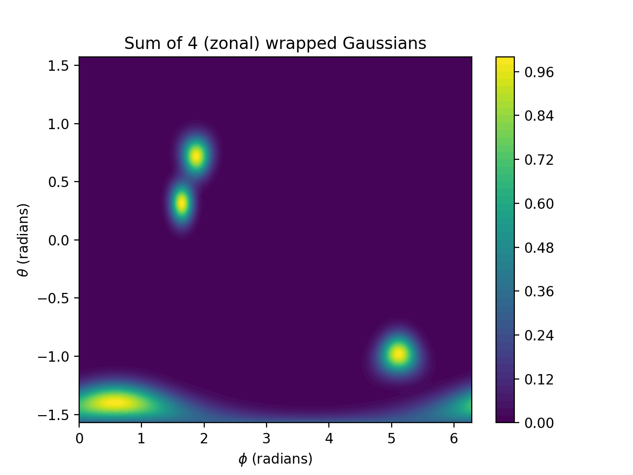
Zonal: \(d(\mathbf{z},\mathbf{x})=\langle\mathbf{z},\mathbf{x}\rangle, \; \forall \mathbf{z},\mathbf{x}\in\mathbb{S}^{N-1}.\) Note that in this case the two point sets must be on the hypersphere \(\mathbb{S}^{N-1}.\)

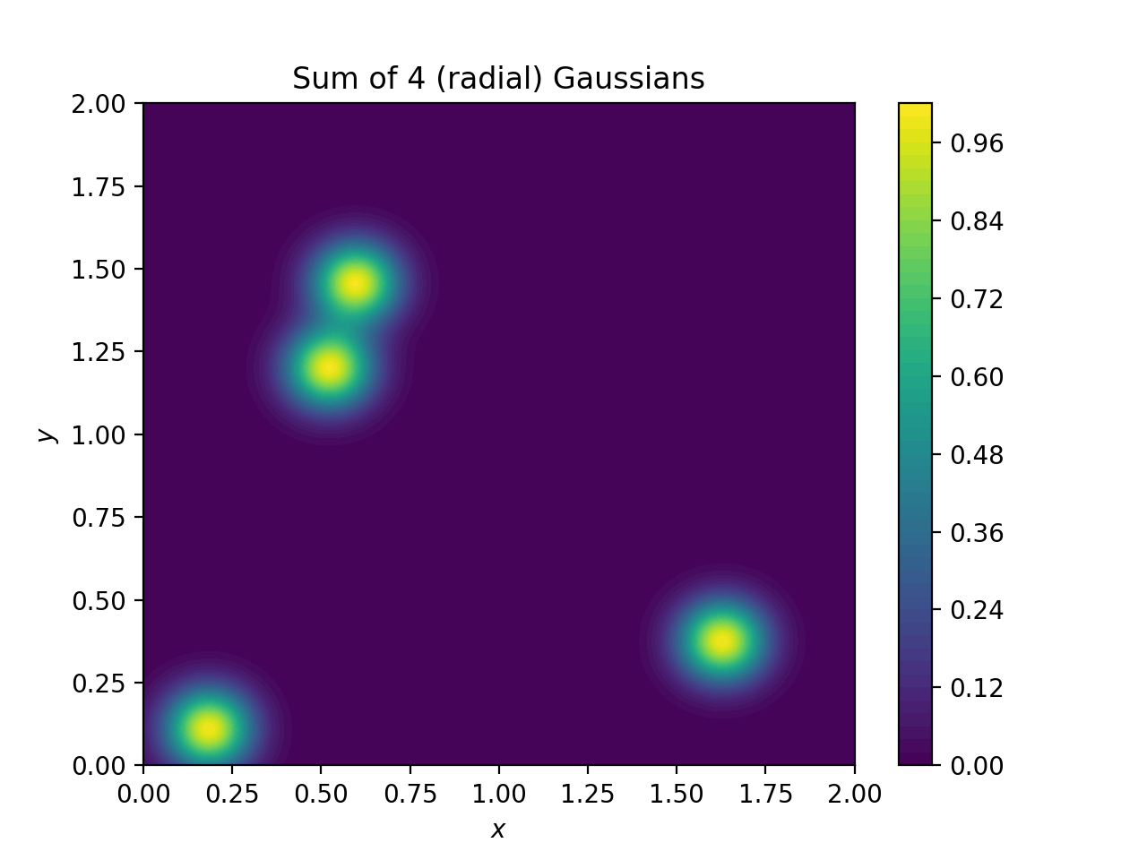
This matrix is useful for sampling sums of radial/zonal functions. Indeed, if \(f(\mathbf{z})=\sum_{k=1}^K\alpha_k\varphi(d(\mathbf{z},\mathbf{x}_k))\), then we have

\[\begin{split}\left[\begin{array}{c}f(\mathbf{z}_1)\\\vdots\\ f(\mathbf{z}_L) \end{array}\right]=\left[\begin{array}{ccc} \varphi(d(\mathbf{z}_1,\mathbf{x}_1)) & \cdots & \varphi(d(\mathbf{z}_1,\mathbf{x}_K))\\\vdots & \ddots & \vdots\\\varphi(d(\mathbf{z}_L,\mathbf{x}_1)) & \cdots & \varphi(d(\mathbf{z}_1,\mathbf{x}_K))\end{array}\right]\left[\begin{array}{c}\alpha_1\\\vdots\\ \alpha_K \end{array}\right].\end{split}\]

Examples

>>> rng = np.random.default_rng(seed=1)
>>> sigma = 1 / 12
>>> func = lambda x: np.exp(-x ** 2 / (2 * sigma ** 2))
>>> max_distance = 3 * sigma
>>> samples1 = np.linspace(0, 2, 10); samples2 = rng.random(size=3)
>>> MDMOp1 = MappedDistanceMatrix(samples1=samples1, samples2=samples2, function=func,max_distance=max_distance, operator_type='sparse', n_jobs=-1)
>>> MDMOp2 = MappedDistanceMatrix(samples1=samples1, samples2=None, function=func,max_distance=max_distance, operator_type='sparse', n_jobs=-1)
>>> MDMOp3 = MappedDistanceMatrix(samples1=samples1, samples2=samples2, function=func, operator_type='dense')
>>> MDMOp4 = MappedDistanceMatrix(samples1=samples1, samples2=samples2, function=func, operator_type='dask')
>>> type(MDMOp1.mat), type(MDMOp3.mat), type(MDMOp4.mat)
(<class 'scipy.sparse.csr.csr_matrix'>, <class 'numpy.ndarray'>, <class 'dask.array.core.Array'>)
>>> MDMOp1.mat.shape, MDMOp2.mat.shape
((10, 3), (10, 10))
>>> MDMOp3.mat
array([[6.43689834e-009, 5.64922608e-029, 2.23956473e-001],
       [2.38517543e-003, 2.61112241e-017, 6.44840995e-001],
       [7.21186665e-001, 9.84802612e-009, 1.51504434e-003],
       [1.77933914e-001, 3.03078296e-003, 2.90456923e-009],
       [3.58222996e-005, 7.61104282e-001, 4.54382719e-018],
       [5.88480228e-012, 1.55961419e-001, 5.80023464e-030],
       [7.88849171e-022, 2.60779757e-005, 6.04161441e-045],
       [8.62858845e-035, 3.55806811e-012, 5.13504354e-063],
       [7.70139186e-051, 3.96130538e-022, 3.56138512e-084],
       [5.60896038e-070, 3.59870356e-035, 2.01547509e-108]])
>>> alpha = rng.lognormal(size=samples2.size, sigma=0.5)
>>> beta = rng.lognormal(size=samples1.size, sigma=0.5)
>>> MDMOp1 * alpha
array([0.27995783, 0.8060865 , 0.37589858, 0.09274313, 1.19684992,
       0.24525208, 0.        , 0.        , 0.        , 0.        ])
>>> MDMOp2 * beta
array([0.80274037, 1.39329178, 1.27124579, 1.22168244, 1.08494933,
       1.36310926, 0.7558366 , 0.96398702, 0.85066284, 1.37152693])
>>> MDMOp3 * alpha
array([2.79957838e-01, 8.07329704e-01, 3.77792488e-01, 9.75090904e-02,
       1.19686859e+00, 2.45252084e-01, 4.10080770e-05, 5.59512490e-12,
       6.22922262e-22, 5.65902486e-35])
>>> MDMOp4 * alpha
array([2.79957838e-01, 8.07329704e-01, 3.77792488e-01, 9.75090904e-02,
       1.19686859e+00, 2.45252084e-01, 4.10080770e-05, 5.59512490e-12,
       6.22922262e-22, 5.65902486e-35])
>>> np.allclose(MDMOp3 * alpha, MDMOp4 * alpha)
True

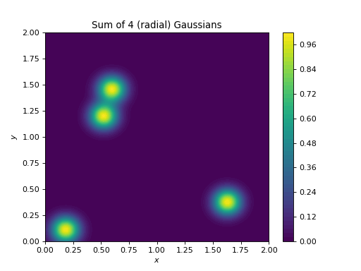
import numpy as np
import matplotlib.pyplot as plt
from pycsou.linop.sampling import MappedDistanceMatrix

t = np.linspace(0, 2, 256)
rng = np.random.default_rng(seed=2)
x,y = np.meshgrid(t,t)
samples1 = np.stack((x.flatten(), y.flatten()), axis=-1)
samples2 = np.stack((2 * rng.random(size=4), 2 * rng.random(size=4)), axis=-1)
alpha = np.ones(samples2.shape[0])
sigma = 1 / 12
func = lambda x: np.exp(-x ** 2 / (2 * sigma ** 2))
MDMOp = MappedDistanceMatrix(samples1=samples1, samples2=samples2, function=func, operator_type='dask')
plt.contourf(x,y,(MDMOp * alpha).reshape(t.size, t.size), 50)
plt.title('Sum of 4 (radial) Gaussians')
plt.colorbar()
plt.xlabel('$x$')
plt.ylabel('$y$')

(Source code, png, hires.png, pdf)

../../_images/pycsou-linop-sampling-4.png

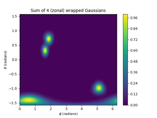
import numpy as np
import matplotlib.pyplot as plt
from pycsou.linop.sampling import MappedDistanceMatrix

rng = np.random.default_rng(seed=2)
phi = np.linspace(0,2*np.pi, 256)
theta = np.linspace(-np.pi/2,np.pi/2, 256)
phi, theta = np.meshgrid(phi, theta)
x,y,z = np.cos(phi)*np.cos(theta), np.sin(phi)*np.cos(theta), np.sin(theta)
samples1 = np.stack((x.flatten(), y.flatten(), z.flatten()), axis=-1)
phi2 = 2 * np.pi * rng.random(size=4)
theta2 = np.pi * rng.random(size=4) - np.pi/2
x2,y2,z2 = np.cos(phi2)*np.cos(theta2), np.sin(phi2)*np.cos(theta2), np.sin(theta2)
samples2 = np.stack((x2,y2,z2), axis=-1)
alpha = np.ones(samples2.shape[0])
sigma = 1 / 9
func = lambda x: np.exp(-np.abs(1-x) / (sigma ** 2))
MDMOp = MappedDistanceMatrix(samples1=samples1, samples2=samples2, function=func,mode='zonal', operator_type='sparse', max_distance=3*sigma)
plt.contourf(phi, theta, (MDMOp * alpha).reshape(phi.shape), 50)
plt.title('Sum of 4 (zonal) wrapped Gaussians')
plt.colorbar()
plt.xlabel('$\\phi$ (radians)')
plt.ylabel('$\\theta$ (radians)')

(Source code, png, hires.png, pdf)

../../_images/pycsou-linop-sampling-5.png

See also

GeneralisedVandermonde

__init__(samples1: numpy.ndarray, function: Callable, samples2: Optional[numpy.ndarray] = None, mode: str = 'radial', max_distance: Optional[float] = None, dtype: type = <class 'numpy.float64'>, chunks: Union[str, int, tuple, None] = 'auto', operator_type: str = 'dask', verbose: bool = True, n_jobs: int = -1, joblib_backend: str = 'loky', ord: float = 2.0, eps: float = 0)[source]¶

Parameters

samples1 (np.ndarray) – First point set with shape (L,N).
function (Callable) – Function \(\varphi: \mathbb{R}_+\to \mathbb{C}\) to apply to each entry of the distance matrix.
samples2 (Optional[np.ndarray]) – Optional second point set with shape (K,N). If None, samples2 is equal to samples1 and the operator symmetric.
mode (str) – How to compute the distances. If 'radial', the Euclidean distance with respect to the Minkowski norm \(\|\cdot\|_p\) is used. \(p\) is specified via the parameter ord and has to meet the condition 1 <= p <= infinity. If 'zonal' the spherical geodesic distance is used.
max_distance (Optional[np.float]) – Support of the function \(\varphi\). Must be specified for sparse representation.
dtype (type) – Type of input array.
chunks (Union[str, int, tuple, None]) – Chunk sizes for Dask representation.
operator_type (str) – Internal representation of the operator: 'dense' represents the operator as a Numpy array, 'dask' as a Dask array, 'sparse' as a sparse matrix. Dask arrays or sparse matrices can be more memory efficient for very large point sets.
verbose (bool) – Verbosity for parallel computations (only for sparse representations).
n_jobs (int) – Number of cores for parallel computations (only for sparse representations). n_jobs=-1 uses all available cores.
joblib_backend (str) – Joblib backend (more details here).
ord (float) – Order of the norm for mode='radial'. ord must satisfy 1<= ord <=infty.
eps (float) – Parameter for approximate nearest neighbours search when mode='sparse'.

Raises

ValueError – If mode is invalid or if operator_type is 'sparse' but max_distance=None.

get_sparse_mdm() → scipy.sparse.csr.csr_matrix[source]¶

Form the Mapped Distance Matrix as a sparse matrix.

Returns: Sparse Mapped Distance Matrix.
Return type: sparse.csr_matrix

get_dask_mdm() → dask.array.core.Array[source]¶

Form the Mapped Distance Matrix as a dask array.

Returns: Mapped Distance Matrix as a Dask array.
Return type: da.core.Array

get_dense_mdm() → numpy.ndarray[source]¶

Form the Mapped Distance Matrix as a dense Numpy array.

Returns: Mapped Distance Matrix as a Numpy array.
Return type: np.ndarray